Paper #1, Part 1: What Does It Mean for a Computer to 'See' a Picture?

Where we are: the beginning. This series builds up, one idea at a time, to how a computer learns to recognize what is in an image.

We’re going to spend this series working through CS231n, the course number of Stanford’s free class on how computers learn to see. It’s a foundational course in deep learning, the kind of course that builds the intuition you need before tackling dense research papers. It also sits at the start of a famous reading list that Ilya Sutskever (a co-founder of OpenAI and one of the researchers behind ChatGPT) is said to have given John Carmack (the programmer behind the video games Doom and Quake).

What We’re Building Is a Function

Here’s the goal, in one sentence: everything in this series is aimed at building a function.

The first function most people meet is y = mx + b. It takes a number x, does some arithmetic, and hands back a number y: give it an input, get an output.

What we’re going to build is the same idea, just bigger. The input, x, is a picture (which, as the next section shows, is just a grid of numbers). The output, y, is a guess about what the picture shows, like “dog”. We find this function by showing it many pictures whose answers we already know and adjusting it until its guesses are usually right, so that it then works on new pictures it has never seen. The finished function is called a model.

This is the opposite of how computer vision used to work. For decades, getting a computer to recognize a dog meant a person deciding, by hand, what to look for: fur, floppy ears, four legs, then writing code to spot those clues. That is enormously hard to get right, because a dog can appear at any angle, in any lighting, against any background. We take the other path: instead of choosing the clues ourselves, we show the function many labeled examples and let it work out what to look for on its own.

That is all a model is: a picture goes in, a guess comes out, and in between is a function we built from examples. Everything else in this series (turning input pictures into numbers the function can work with, scoring them, measuring the mistakes, improving the guesses, and turning the output numbers back into a result a person can understand and finds useful) is detail in service of building that one function.

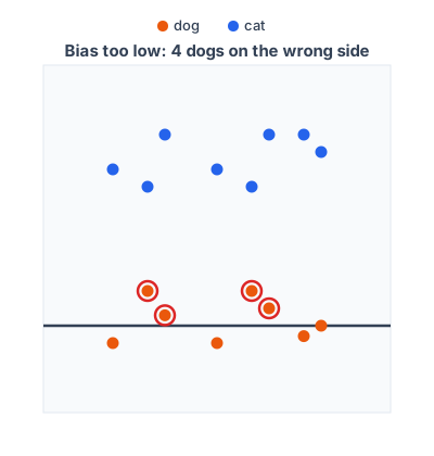
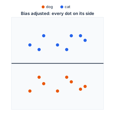
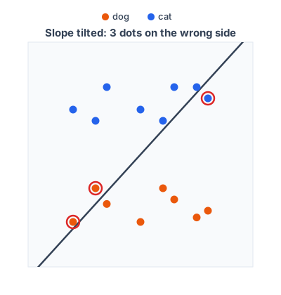
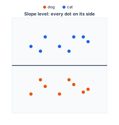
To see what “adjusting it until its guesses are right” looks like, picture each example as a dot on a graph, blue for cats and orange for dogs, where each axis is some measurement of the image (not the picture-in or guess-out from before, just two numbers that place each image on the graph), so similar pictures sit near each other. The model becomes a dividing line: “cat” on one side, “dog” on the other. A dot on the correct side is a right guess; a dot on the wrong side is a mistake.

That dividing line has the same straight-line shape as y = mx + b. Training adjusts its two knobs, the slope m and the intercept b (also called the bias), to push more dots onto their correct side; the model’s guess for a new image is just which side of the line its dot lands on.

Slide the bias up or down, and the same-angle line separates the dots well or badly:

Tilt the slope, and again it separates them well or badly:

Nudging those two knobs until more dots end up on the correct side is how training works. Sorting labeled dots into their groups like this even has a name, classification, and it is what the next several posts are about.

This cat-versus-dog classifier is the running example for the whole series. Each new idea we meet, from scoring images to measuring mistakes to full convolutional networks, we’ll bring back to the same question: is this picture a cat or a dog?

Everything that comes after this is the same idea, scaled up for harder data: more capable functions, and better ways to train them, so the boundary can handle messy, real-world images instead of two tidy groups of dots. And any change we make to the function (add curves, crooks, or corners; combine many lines instead of one; give it far more knobs to tune) is completely fine, as long as it makes the function better at predicting pictures it hasn’t seen. It’s our function; we can build it however we want.

But before we build anything, we need to ask a basic question: what does a computer actually receive when we hand it a picture?

A Picture Is Just Numbers

A human brain sees a photo and almost instantly knows it contains a dog. It happens without any conscious thought. The image “makes sense” to a person.

A computer doesn’t work that way. A computer can only work with numbers. (Underneath, even those numbers are stored as tiny on-off switches, but thinking of them as numbers is enough for our purposes.) So before a computer can “understand” an image at all, the image has to be converted into numbers. By “understand” we just mean: map the numbers to the correct label. The computer isn’t doing anything like human comprehension.

Every image on a screen is stored as a grid of pixels, tiny colored squares. If the image is 800 pixels wide and 600 pixels tall, that’s an 800 × 600 grid. Each pixel’s color is written down as three numbers: how much red, how much green, and how much blue it contains (the RGB system). Each of those three numbers is a whole number from 0 (none of that color) to 255 (as much as possible).

So an 800 × 600 image is stored as an 800 × 600 × 3 grid of numbers. That’s 1.44 million numbers to represent one photo. (The 0 to 255 range is the most common convention. Some formats allow a wider range. And neural networks (programs that learn from examples, which we’ll meet later in this series) often shrink these values down to sit between 0 and 1, because that helps them learn more reliably.)

Scrolling through photos on a phone means shuffling around millions of numbers. And compressing an image for email (that is, shrinking its file size so it uploads faster and takes up less storage) means playing one of two tricks with those numbers:

• Write the repeats as shorthand. A clear blue sky means the same three numbers repeated thousands of times in a row. A format can store that as, in effect, “sky color, five thousand times” instead of writing it out five thousand times. Reversing the shorthand gives back every original number exactly. This is a simplified version of what is called “lossless compression” (no detail is lost; you can rebuild the original exactly): real formats like PNG use a more elaborate method (called DEFLATE), but the idea of storing repeats compactly is the same.
• Throw away detail the eye won’t miss. A format can also smooth over tiny differences between neighboring pixels and store the simpler result. The numbers that come back are close to the originals, but not identical. This is called lossy compression, it’s what JPEG files do, and it’s why JPEGs are so small.

Either way, compressing a picture is just doing arithmetic on a grid of numbers.

This is where computers start. Not with “a picture of a dog.” With a giant grid of numbers.

The Numbers, Up Close

A small example makes this concrete. Here is a 64 × 64 pixel cartoon dog:

This little dog is a 64 × 64 grid: about twelve thousand numbers. That’s enough for a blocky cartoon but nowhere near enough for the fur, whiskers, and shadows of a real photo. A phone photo is the exact same kind of thing, just bigger. A 12-megapixel photo is a grid of about 36 million numbers, roughly three thousand times more than our dog. More numbers means finer detail, but the structure never changes.

And here is the exact same picture, as a file of readable numbers: dog.ppm.txt.

That file is a real image format (called “plain PPM”) that image editors such as the free program GIMP will open as a picture. But because it stores its numbers as ordinary text, it is also readable as-is: open it in a browser or a text editor and the numbers are right there.

Things to look for in the file:

• After the short header, every group of three numbers is one pixel: red, green, blue.
• The file starts with 170 210 240 repeated over and over. That’s the sky: some red, more green, a lot of blue makes light blue. (It’s also exactly the kind of repetition that the lossless shorthand trick from earlier collapses.)
• Further down, the numbers change to 100 60 30. More red than green, very little blue: that’s the dark brown of the dog’s ears.
• Further still come 25 25 25 (the nearly-black eyes and nose) and 230 120 140 (the pink tongue).

The dog in the picture and the wall of numbers are the same thing. Every method in the rest of this series works on those numbers.

What’s Next

In the next post, we ask the question that CS231n spends a semester answering: given a grid of numbers like this one, how can a computer decide what the picture shows? It sounds simple. Seven specific things make it surprisingly hard, starting with the fact that the same dog photographed in different lighting produces a completely different grid of numbers.

New terms from this series are collected in the glossary.