Paper #5: Dilated Convolutions, a Filter with Gaps
A dilated convolution spaces out the positions a filter reads, so the same few weights cover a wider area. Stack a few with growing gaps, and the area each output sees grows exponentially, while the map never shrinks.
Where we are: the last post showed that classification networks shrink their maps so later layers can see wide areas, and that segmentation needs the wide view without the shrinking. This post covers the paper’s tool for that: the dilated convolution.
A filter on a single row
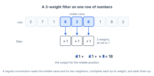
Start with one row of 9 numbers and a filter with 3 weights, all set to 1, so the filter just adds up the values it lands on. The row is 2, 7, 1, 8, 2, 8, 1, 8, 2, and the filter is centered on the middle value, 2.
A regular convolution centered on the middle value reads it and its two neighbors:
A dilated convolution reads values that are a fixed distance apart instead. That distance is the dilation.
- Dilation 1 (a regular convolution) reads the 3 values next to each other: 8 + 2 + 8 = 18. It spans 3 positions.
- Dilation 2 reads every 2nd value: 1 + 2 + 1 = 4. It spans 5 positions.
- Dilation 4 reads every 4th value: 2 + 2 + 2 = 6. It spans 9 positions, the whole row.
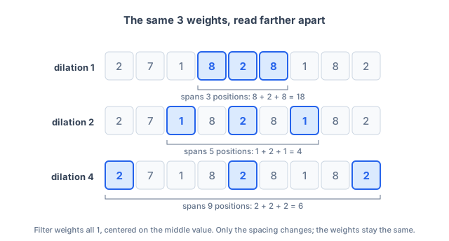
The filter has the same 3 weights every time. Only the spacing between the positions it reads changes. No larger filter is built; the convolution just reads its inputs farther apart.
Why the map does not shrink
The filter then slides one position at a time and produces an output at every position, the same as a regular convolution. Near the edges, where some taps would fall off the row, the row is padded. The output row has as many values as the input row.
That is the difference from pooling and striding. A 2 × 2 pooling step turns a 56 × 56 map into a 28 × 28 map; a dilated convolution with dilation 2 turns a 56 × 56 map into another 56 × 56 map, while still reading from a wider area.
In two dimensions
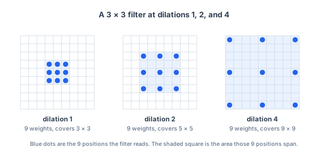
On an image or a feature map, a 3 × 3 filter has 9 weights. At dilation 1 its taps sit next to each other and cover a 3 × 3 area. At dilation 2 they spread out to cover 5 × 5, with a gap between each pair. At dilation 4 they cover 9 × 9. It is still 9 weights each time.
Stacking them
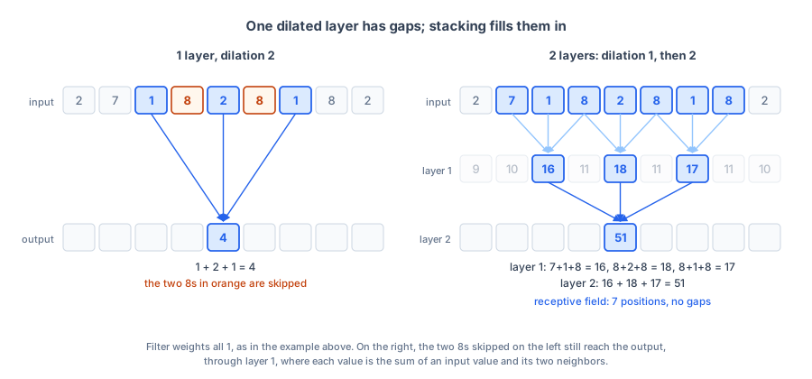
With one layer, the wider view has gaps: dilation 2 skips every other value. Stacking layers fills in the gaps and widens the view much faster. Each layer reads from the layer before it, and each position in that earlier layer already summarizes an area of the image. The area a single output depends on is called its receptive field.
The paper’s Figure 1 stacks three 3 × 3 layers with dilations 1, 2, and 4:
- Layer 1, dilation 1: each output depends on a 3 × 3 area.
- Layer 2, dilation 2: each output reads 3 × 3 positions from layer 1, spaced 2 apart, so they span 5 × 5 positions, and each of those already covers 3 × 3. Together: 7 × 7.
- Layer 3, dilation 4: by the same reasoning, 15 × 15.
The figure below shows one filter in each layer. Dark blue squares are the 9 positions the filter reads; the yellow area is how much of the input its output depends on. Lines show which values are added up to make the next layer’s value.
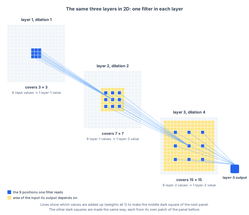
Doubling the dilation at each layer roughly doubles the receptive field each time. In the paper’s words, “the receptive field grows exponentially while the number of parameters grows linearly”: every layer adds the same 9 weights per filter, but the area it covers keeps doubling. Three regular 3 × 3 layers, with the same number of weights, would cover only 7 × 7, against 15 × 15 for the dilated stack.
The context module in a later post uses dilations 1, 1, 2, 4, 8, 16, which gives receptive fields of 3 × 3, 5 × 5, 9 × 9, 17 × 17, 33 × 33, and 65 × 65 after each layer. Those are the numbers in the 1st post.
An old idea under a new name
The operation itself was not new. It appears in the “algorithme à trous,” French for “algorithm with holes,” a method for analyzing signals with wavelets from 1987. DeepLab, a segmentation network from 2015, also used it. The authors chose the name “dilated convolution” and built a network that, in their words, “systematically uses dilated convolutions for multi-scale context aggregation,” meaning combining information from both small and large areas around each position.
What’s next
The next post covers how the authors used this: first to stop VGG-16 from shrinking its last maps, and then to build a small “context module” that stacks dilated layers to see wide areas at full resolution.