Paper #5: From One Label to Every Pixel

Where we are: Paper #4, Identity Mappings, finished the thread about making networks deeper. Paper #5 changes the task.

What the papers so far have done. Papers #2–4 (AlexNet, ResNet, Identity Mappings) all improved classification: given a whole image, name what’s in it. The output is one label per image, like “cat.”

What Paper #5 is for. “Multi-Scale Context Aggregation by Dilated Convolutions” (Fisher Yu and Vladlen Koltun, ICLR 2016) works on semantic segmentationlabeling every pixel of an image with a category, such as road, car, or sky, instead of giving the whole image one label.: label every pixel, such as “this pixel is road, this one is a pedestrian, this one is sky.” The output is a full-size map, not one word. This is what a self-driving car needs from a camera image, and the paper tests on street-scene datasets (CamVid, KITTI, Cityscapes) as well as PASCAL VOC.

The problem it solves. Classification networks shrink the image as it passes through them, from 224 × 224 down to 7 × 7 in ResNet. That’s fine for producing one label, but it throws away the detail needed to label each pixel. The authors question whether “severe intermediate downsampling was truly necessary.” Their tool is the dilated convolutiona convolution whose filter taps are spaced apart, so the same number of weights covers a wider area of the input without shrinking it.: a filter with gaps between its taps. It sees a wider area without shrinking the maps or adding weights, and stacking them makes the area seen grow exponentially (3×3, 5×5, 9×9, 17×17…). The network keeps much more detail and still sees enough context to tell a road from a sidewalk.

Where it has been used. Labeling every pixel is useful well beyond street scenes: outlining organs and tumors in medical scans, mapping roads and buildings in satellite images, and separating a person from the background in photo and video tools. The dilated convolution itself also moved beyond images. DeepMind’s WaveNet (2016), which generates speech, and ByteNet (2016), which translates text, both stack dilated convolutions to take in long stretches of input, and both cite this paper. The last post has the details.

A short history

Labeling every pixel was not a new goal in 2015.

• 2004–2013, hand-designed features. Methods built on features a person chose, much like classification before AlexNet. The paper cites work from 2004 on labeling images at several scales, TextonBoost (Shotton et al., 2009), and SuperParsing (2013).
• 2013, an early convolutional network. Farabet et al., with Yann LeCun, learned the features for scene labeling instead of designing them.
• 2015, classification networks adapted. FCN and DeepLab took networks like VGG-16 and changed them to output a map instead of one label. The next post covers how.
• 2015–2016, this paper. Yu and Koltun asked whether the shrinking those adapted networks kept was needed at all.

FCN (Long et al., 2015) is usually credited as the paper that first turned a classification network into a segmentation network. So why does the 30 papers list include Yu and Koltun’s paper instead? There’s no way to know for sure: Ilya Sutskever, who reportedly put the list together, hasn’t publicly explained his picks. One possible reason is that the main technique from Yu and Koltun’s paper carried over to other kinds of data. Within a year, WaveNet used dilated convolutions for audio and ByteNet used them for text, and the list itself moves from images to sequences right after this paper.

What a segmentation looks like

A classification network looks at a street photo and outputs one answer, such as “car.” A segmentation network outputs a 2nd image the same size as the photo, where every pixel holds a category instead of a color. The pixels covering the car say “car,” the ones covering the road say “road,” and so on. Drawn with one color per category, it looks like a coloring-book version of the photo.

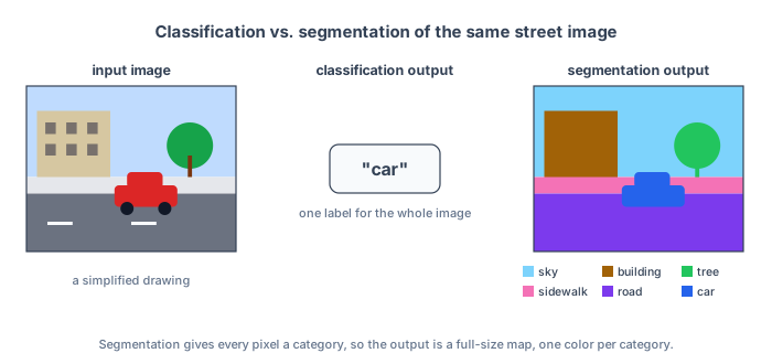
The paper calls this “dense prediction”: a prediction at every position, as opposed to one prediction for the whole image.

The categories are fixed in advance. Each dataset comes with its own list, such as 21 for PASCAL VOC (20 kinds of objects plus “background”) or 11 for the street scenes in CamVid, and people label every pixel of the training images with one of them. The network is built with one output per category and learns what each one looks like; it doesn’t decide which categories exist.

Segmentation needs two things at once:

• Detail. The boundary between the car and the road has to land on the right pixels.
• Context. A gray patch could be road, sidewalk, or a building wall. Telling them apart often means looking well beyond the patch itself, at what is around it.

Image classification networks, like the ones in Papers #2–4, are built for context and give up detail along the way. Paper #5’s network starts from VGG-16, a classification network of the same kind from 2014, keeping its layers and trained weights, and changes it to keep the detail.

How a segmentation is scored

The paper scores its results with mean IoUa segmentation score: for each category, the overlap between the predicted and true regions divided by their combined area, averaged over the categories., short for mean intersection over union. For one category, say road:

• the intersection is the set of pixels the network called road that are road in the true labels;
• the union is every pixel that is road in either the prediction or the true labels.

With made-up numbers: the true road covers 100 pixels, the network labels 90 pixels as road, and 80 of those are correct. So it missed 20 road pixels, and labeled 10 other pixels as road by mistake.

IoU = overlap ÷ combined area = 80 ÷ (100 + 90 − 80) = 80 ÷ 110 ≈ 73%

Adding the two areas, 100 + 90 = 190, counts the 80 overlapping pixels twice, so they are subtracted once: 190 − 80 = 110. A perfect prediction scores 100%. Missing road pixels and labeling non-road pixels as road both lower the score. Mean IoU averages this over all the categories, so a small category like “pedestrian” counts as much as a large one like “road.”

You might ask, why not just count the share of all pixels in the image that got the right label? That’s called “pixel accuracy” or “global accuracy,” and it is sometimes reported as well. The problem is that large regions dominate it. In a street scene, road, sky, and buildings cover most of the pixels, and pedestrians cover very few. If road covers 70% of an image, a network that labels every pixel “road” scores 70% pixel accuracy without finding a single pedestrian.

Mean IoU scores each category separately before averaging, so the same network would get 70% on road and 0% on every other category, and with 11 categories, as in CamVid, its mean IoU would be about 6%. For a self-driving car, that difference matters: missing a pedestrian is far more costly than mislabeling a patch of sky. Mean IoU doesn’t weight pedestrians more than sky, but it counts every category equally, so a network can’t score well while ignoring the small ones.

Mean IoU is the standard way of scoring segmentation, but there are other ways as well. Instance-level IoUordinary IoU lets a big, close car count far more than a small, distant pedestrian, because the car covers more pixels; instance-level IoU weights each object's pixels by its size, so small, distant objects count about as much as large ones., frequency-weighted IoUIoU for each category, weighted by how many pixels the category covers, so large categories like road and sky count more. The FCN paper reports it alongside mean IoU., and custom, task-specific weightsscores with weights chosen to match a particular system's costs, such as counting a missed pedestrian much more heavily than a mislabeled tree. There is no single standard for this, and published benchmarks rarely use it. have all been used. Another approach leaves the score alone and changes the training loss instead. A class-weighted loss makes each mistake on a rare category, like pedestrians, cost more during training, so the network pays more attention to it.

The datasets

• PASCAL VOC 2012: everyday photos with 20 object categories, such as people, cats, cars, and chairs, plus background. This is where the paper runs most of its experiments.
• CamVid, KITTI, and Cityscapes: street scenes recorded from cars, with categories like road, sidewalk, building, car, and pedestrian. Cityscapes images are 2048 × 1024 pixels.

What’s next

The next post looks at why classification networks shrink the image in the first place, and what earlier segmentation networks did to get the detail back.