Paper #5: Why Classification Networks Shrink the Image
Classification networks shrink their feature maps on purpose: it lets later layers see wide areas cheaply. For one label that costs nothing. For a label at every pixel, it throws away the detail the answer needs.
Where we are: the last post described segmentation: a label for every pixel, which needs both fine detail and a wide view of the surroundings. This post covers why classification networks give up the detail, and what earlier segmentation networks did about it.
Shrinking on purpose
A classification network shrinks its feature maps several times on the way to the answer. Two steps do the shrinking:
- Pooling, covered in Paper #1’s post on pooling: each 2 × 2 patch of a map is replaced by one value, so the map’s width and height are halved.
- Striding: a convolution that moves 2 positions at a time instead of 1, which also halves the width and height.
ResNet, from Paper #3, does this five times: a 224 × 224 image becomes maps of 112 × 112, then 56 × 56, 28 × 28, 14 × 14, and finally 7 × 7.
The shrinking is there for a reason. Each layer’s filters look at a small patch, 3 × 3 positions in most of these networks. On a full-size map, a 3 × 3 patch covers 3 × 3 pixels of the image. On a map that has been halved five times, each position stands for a 2⁵ × 2⁵ = 32 × 32 block of pixels, so the same 3 × 3 filter covers at least a 96 × 96 area. Shrinking is a cheap way to let later layers see large parts of the image, which they need to recognize whole objects.
Fine for one label, not for every pixel
For classification, the final answer is one word for the whole image. Where exactly the cat is does not matter, only that there is one. By the 7 × 7 stage, each position summarizes a large region, and ResNet then averages the 49 positions into one summary before the final layer. Nothing about the answer depends on the detail that was given up.
For segmentation, the answer is a label at every pixel, so the detail isn’t something we can throw away. A 7 × 7 map has 49 positions for a 224 × 224 image with 50,176 pixels. Each position has to stand for a 32 × 32 block. If a block contains part of a car and part of the road, that one position cannot say where the edge between them runs.
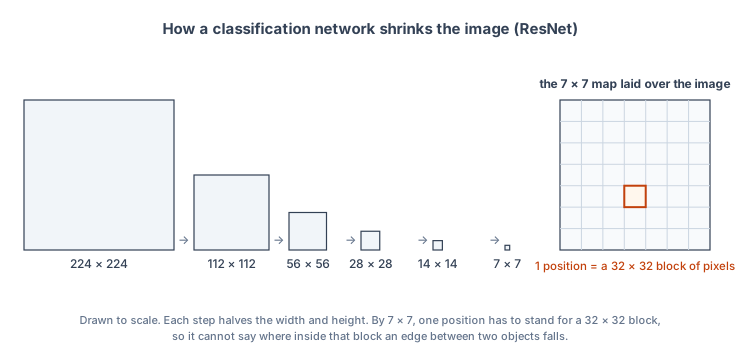
So a segmentation network needs the wide view that shrinking provides and, at the same time, the detail that shrinking throws away.
What earlier networks did
By 2015, the best segmentation systems started from classification networks such as VGG-16 and adapted them. The paper describes two main approaches.
Shrink, then scale back up. Keep the classification network’s shrinking, then add layers at the end that enlarge the small maps back to full size.
Look at several sizes of the image. Feed the network rescaled copies of the image, small and large, and combine the predictions from each. The paper questions whether this is needed either: running the network several times on rescaled copies of the image is extra work, to make up for detail the network threw away in the first place.
Both approaches keep the shrinking. Enlarging a 7 × 7 map back to 224 × 224 cannot restore detail that is no longer in it; it can only spread what is left over more pixels. Some versions also feed in the earlier, larger maps, which still have the detail, but that detail comes from those maps, not from the shrunk one.
The question the paper asks
The authors put the problem this way: the upsampling approach “leaves open the question of whether severe intermediate downsampling was truly necessary.”
In other words: if the only reason for shrinking was to let later layers see wide areas, is there another way to get the wide view without shrinking at all? The paper’s answer is the dilated convolution, which spaces out the positions a filter reads so that it covers a wide area of a full-size map, using the same number of weights.
What’s next
The next post covers how a dilated convolution works, starting with a single row of numbers, and how stacking a few of them makes the area each output sees grow quickly.