Paper #1, Part 13: Pooling and Stacking (From Edges to Objects)

Where we are: convolutions find small local patterns anywhere in an image (Part 12). Now we stack them, together with pooling, to build from edges all the way up to whole objects.

After a convolutionslide a small filter across the image to find a pattern anywhere. layer, feature mapsthe grid of responses a filter produces as it slides over the input. are the same size as the input (or slightly smaller). If the input is 224×224, the output might be 222×222.

Apply another convolution, get 220×220. Each layer shaves off only a little, so the maps stay large for many layers, the computation piles up, and each convolution still only sees a small local patch.

Pooling solves this. It downsamples: takes a region (like 2×2) and outputs a single value. Common pooling: max pooling. Take the maximum value in each 2×2 region.

Input (6×6):
 1  2  3  4  5  6
 7  8  9 10 11 12
13 14 15 16 17 18
19 20 21 22 23 24
25 26 27 28 29 30
31 32 33 34 35 36

Max pooling with non-overlapping 2×2 regions, giving a 3×3 output:
 8 10 12
20 22 24
32 34 36

Output is about half the size in each dimension. A 224×224 map becomes 112×112.

Why Pooling Works

Aggregation: Pooling combines information from a small region into one value. Within that region the exact position stops mattering; what carries forward is mainly whether the feature is present.

Robustness: if a pattern shifts by a pixel or two, max pooling often gives the same result, since the largest value in the window is usually still the largest. That makes the network more tolerant of small shifts, which helps recognition. Picture a spotlight following a singer: as long as the singer stays somewhere inside the circle of light, the audience sees the same bright figure, even as they drift a step left or right. The pooling window is that circle of light for a feature. (The flip side: pooling blurs away exact positions, so it’s less suited to tasks that need to locate things precisely.)

Dimensionality reduction: Smaller feature maps = faster computation.

Wider view: because pooling shrinks the maps, each filtera small grid of weights that detects one pattern (also called a kernel). in the next layer covers more of the original image. A 3×3 filter working on a once-pooled map effectively spans a 6×6 patch of the input; after another round of pooling, wider still. This is what lets deeper layers combine small patterns into bigger ones, which is the hierarchy below.

The Hierarchy

Stacking convolution and pooling layers builds a hierarchy:

Input image (224×224)
  ↓ Conv (detect edges)
  ↓ Pool (224→112)
  ↓ Conv (detect edge combinations, i.e., textures)
  ↓ Pool (112→56)
  ↓ Conv (detect texture combinations, i.e., shapes)
  ↓ Pool (56→28)
  ↓ Conv (detect complex shapes, i.e., object parts)
  ↓ Pool (28→14)
  ↓ Fully connected layers (make the final decision)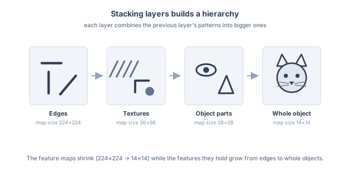

Early layers detect simple features. Later layers detect complex combinations. By the time you reach a fully-connected layera layer where every input connects to every neuron., you’re working with high-level features (combinations that respond to things like shapes and object parts) rather than raw pixels.

That fully-connected layer at the end isn’t a step backward to where we started. Part 12’s objection was to running a fully-connected layer directly on raw pixels: wiring every pixel to every neuronone unit that weights its inputs, adds them up, and applies an activation. takes an enormous number of weightsthe numbers inside the model that it adjusts as it learns. and learns each pattern separately for every position. Convolution and pooling handle that part, scanning locally and reusing the same filters everywhere. But the final decision has to weigh all the evidence together: given every shape and part the network found, anywhere in the image, what is this? That’s a global question, and a fully-connected layer, which connects to everything at once, is suited to it. What changed is what it connects to: a compact set of high-level features, not a raw grid of pixels.

Loosely speaking, a cat classifier ends up responding to a particular combination of these features: certain edges here, certain textures there, together adding up to “cat” (not a rule written in words, but a pattern of numbers that behaves like one).

What’s Next

This hierarchy works, but it’s hard to tell what the network actually learned: its filters are millions of numbers, and looking at those numbers doesn’t reveal what each one detects. Part 14 covers how to visualize and interpret what convolutional networks see.