Paper #1, Part 14: Peeking Inside the Black Box (What Is a CNN Looking At?)
Neural networks learn patterns, but we can't see them directly. Visualization techniques let us peek inside and understand what features a network has learned.
Where we are: we can build convolutional networks that recognize objects (Parts 12 and 13). But what has such a network actually learned? This post is how to look inside and see.
A trained CNN is powerful but opaque. Weights are numbers. Feature maps are high-dimensional arrays. How do you know what the network learned?
Making sense of what a trained network is doing is called interpretability. Its main tool is visualization: techniques that let you inspect the network and see what it learned.
Visualizing Filters
The simplest approach: display the weights of early-layer filters as images.
Early filters in a trained network often look like edge detectors:
- Horizontal line patterns (detect horizontal edges)
- Vertical line patterns (detect vertical edges)
- Diagonal patterns (detect diagonals)
- Blobs and textures
You can literally see what features the network is looking for.
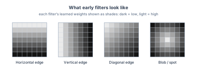
These are illustrations of the idea, not filters from a specific trained network, but real early-layer filters look much like this.
Deeper layers are harder to interpret from their weights alone. A deep filter doesn’t read raw pixels; it reads the many feature maps the layer before it produced. Its weights span that whole stack, so they don’t come together into a single picture you can just look at. Instead of inspecting the weights, you study how the filter behaves: which images make it fire, and which parts of an image it responds to. That’s what the rest of this post does.
Feature Maps
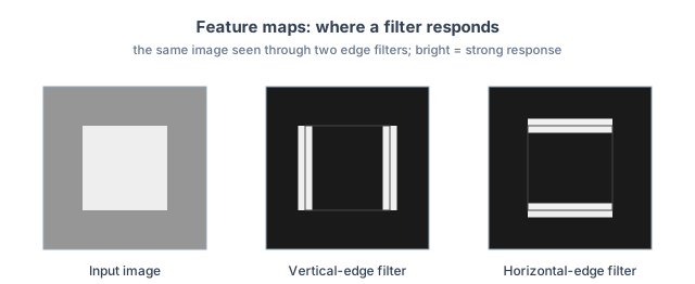
Visualizing a filter’s weights shows what pattern it looks for. A feature map shows where it found that pattern in a particular image.
Recall from Part 12 that when a filter slides across an image, it produces a grid of numbers, one per position, each saying how strongly the filter’s pattern shows up at that spot. (Part 12 called this the filter’s output map; “feature map” is the same thing.) Shown as an image, that grid is bright wherever the pattern is present and dark where it isn’t.
So you can feed a real image through the network and look at the maps it produces. The vertical-edge filter’s map lights up along the vertical edges; the horizontal-edge filter’s map lights up along the horizontal ones:
The maps change character as you go deeper into the network:
- Early maps light up on simple features in specific places: edges, mostly.
- Middle maps light up on textures and small shapes.
- Late maps light up on high-level, task-related features. For a cat classifier, a late map might brighten around the eyes, the ears, or the face, wherever those happen to be in the image.
Reading the maps tells you not just what the network can detect but where it detected it in this particular image. That’s the first step toward the question the next sections ask: which parts of the image actually drove the decision?
Activation Maximization
Ask: “What image would maximally activate this neuron?”
Generate an image that makes a specific neuron fire as strongly as possible. The result is often interpretable: optimize a face-detecting neuron and face-like shapes emerge, though as repeated, dreamlike fragments rather than one clean face.
This uses the same gradient trick as training, but aimed at the image instead of the weights. In training, the network nudges its weights to lower the loss (Part 7); here the weights stay fixed and we nudge the image, to raise the chosen neuron’s activation. Start from random noise, work out which way to tweak each pixel to make the neuron fire a little more, adjust, and repeat.
The resulting images often look strange, full of repeated, swirling patterns, but they reveal what the neuron responds to.
Saliency Maps
Feature maps show where the network sees its features. A saliency map asks a more specific question: for one image and one prediction, which pixels mattered most to the decision?
Here’s the idea. Take a photo the network labels “cat.” Now ask, one pixel at a time: if I brightened or darkened this pixel a little, how much would the “cat” score change? A pixel that barely moves the score didn’t matter much; a pixel that swings it a lot did. That sensitivity, measured for every pixel at once, is the saliency map. (Measuring how much an output shifts when you nudge an input is exactly the gradient from Part 7, taken here with respect to the image rather than the weights.)
Shown as an image, the pixels the score is most sensitive to come out bright, and the ones that barely matter stay dark:
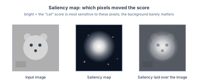
For a well-trained classifier, the hot region often sits on the thing being classified, the animal’s face rather than the background, which is a reassuring sign it’s keying on the right pixels. Saliency maps are noisy, though, as the stray specks in the middle image above show, so treat them as a hint rather than a precise readout.
Why This Matters
Visualization lets you check whether the network learned sensible features. If a cat classifier is keying on cat faces and whiskers, that’s a good sign; if it’s keying on background colors, that’s a warning sign it’s relying on the wrong cue.
Visualization also helps diagnose failures: if the network keeps getting paws wrong, its saliency and feature maps can show whether it’s even looking at the paws, which points you toward a fix (more data, better augmentation, an architecture change).
Interpretability is being able to make sense of what the network is doing and why. And it’s essential for many machine learning applications, especially those that are safety-critical (medical imaging, autonomous driving).
What’s Next
Understanding what a network learned is powerful. But training from scratch is expensive. Part 15 covers transfer learning: reusing a network trained on one task as a starting point for another.