Paper #1, Part 12: Convolutions (Spotting Patterns Anywhere in a Picture)

Where we are: we have the full toolkit for general neural networks (Parts 5 to 11). Now we specialize it for images with a new building block: the convolution.

A fully-connected network connects every pixel to every neuronone unit that weights its inputs, adds them up, and applies an activation., each connection with its own weight, after flattening the image into a long list of pixels.

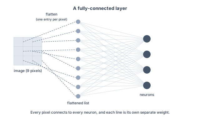
This ignores a key property of images: locality. Important patterns are usually local. An eye is a small region. A texture is a repeating pattern over nearby pixels. A fully-connected layer can’t take advantage of that. By flattening the image into a list, it ignores which pixels are next to which, so a nearby pair of pixels and a far-apart pair look exactly the same to it.

Convolution takes advantage of locality instead: it slides a small filter (like a 3×3 grid) across the image, and at each position computes the dot product between the filter and the image region under it (multiply each filter number by the pixel beneath it, then add them all up).

A Concrete Example

Imagine a 5×5 image and a 3×3 filter:

Image:                Filter:
10 10 10 10 10        0 -1  0
10 50 10 10 10       -1  4 -1
10 10 10 10 10        0 -1  0
10 10 10 10 10
10 10 10 10 10

Place the filter over the top-left corner of the image and multiply element-wise with the 3×3 region it covers:

(10*0 + 10*-1 + 10*0 + 10*-1 + 50*4 + 10*-1 + 10*0 + 10*-1 + 10*0) = 200 - 40 = 160

This gives one output value: 160, which becomes the top-left cell of the output map. The 160 is large because this patch contains the bright spot (50) that this filter responds to. Run the same filter over a flat patch instead (all 10s, with no spot) and it gives 0, because the filter’s weightsthe numbers inside the model that it adjusts as it learns. sum to zero (a +4 and four -1s, with the rest 0s), so they cancel out on any constant patch. So the same filter is selective: a large output where its pattern appears, near zero where it doesn’t. Slide the filter one pixel to the right and repeat. Slide down and repeat. After sliding everywhere, you get a smaller output map: here, a 3×3 map from the 5×5 image.

With a 3×3 filter sliding one pixel at a time and no padding, the output is 2 pixels smaller in each dimension, since the filter can’t slide off the edges. Adding a one-pixel border of zeros around the image, called padding, keeps the output the same size (a larger filter needs a wider border).

What the Filter Learns

The values in the above 3×3 filter are weights, and are learned over repeated rounds of training, just like the weights in a fully-connected layer. After training, filters often learn to detect specific features:

• Edge filters (horizontal, vertical, diagonal edges)
• Texture filters (corners, blobs)
• More complex patterns in deeper layers

Many Filters, One Layer

One filter finds one kind of pattern. But an image has many patterns at once (edges in different directions, textures, colors). So a convolutional layer doesn’t use a single filter; it uses a bank of them, often dozens (say 32), each with its own learned weights and each hunting for a different pattern. Every filter slides across the image and produces its own output map, so a layer with 32 filters turns the input into 32 stacked maps: a 3D block of results. The next layer’s filters then slide over that 3D block of results (each filter spanning the full stack of maps, sliding only across width and height), looking for patterns in those patterns.

Why Convolution Works

Local receptive fields: each output value depends only on a small region of the input, called its receptive field (the part of the input it takes in). A pattern just has to fall within one of these small patches; it doesn’t have to line up with the whole image.

Parameter sharing: The same filter slides everywhere. This dramatically reduces the number of parameters (the learned weights): one small filter is reused across the whole image, instead of a separate weight for every pixel.

A filter works everywhere: because the same filter slides across the whole image, it spots its pattern wherever that pattern appears. Say the network has learned a detector for a dog’s nose: it finds the nose whether it sits in the corner or dead center, because the same detector runs at every position. A fully-connected layer would instead have to learn “nose” separately for each position, needing far more weights and examples of noses in every spot; if it had trained only on centered noses, it would miss one in the corner. Convolution learns a pattern once and reuses it everywhere. (A later step called pooling summarizes each region, which makes the network less sensitive to exactly where a pattern appears.)

Together, these let a convolutional layer find patterns anywhere in an image with far fewer parameters than a fully-connected layer.

Worth making explicit, because it’s a common misconception: this advantage comes from locality and sharing, not from the filter being a 2D grid. The 2D shape matters only because it lets the filter line up with a 2D image neighborhood; a 1D convolution does the same job for 1D data like audio, and a fully-connected layer could in principle learn the same patterns, just far less efficiently and without reusing them across positions.

What’s Next

A single convolution only looks at a small patch, so it can only find small, local patterns: an edge here, a texture there. But recognizing a whole object means combining many of those small patterns across the entire image. A cat isn’t in any one patch; it’s edges, fur, ears, and eyes spread across the picture.

So we need later layers to take in larger and larger regions, building small patterns up into bigger ones: edges into textures, textures into shapes, shapes into objects. The obstacle is that stacking convolutions barely shrinks the maps (224×224 becomes 222×222), so each filter’s view stays local and the computation piles up.

Part 13 covers the fix: pooling. It shrinks the maps as you go, which both cuts the computation and widens what each later layer can see, so stacking convolution and pooling together builds the edges-to-objects hierarchy.