Paper #1, Part 5: Giving the Computer a Scorecard (Linear Classifiers)

Where we are: nearest neighbor just memorized images (Part 3), and we have a way to test a classifier without cheating (Part 4). Now we build the first classifier that truly learns: the linear classifier.

Nearest neighbor failed because it relies on pixel-level similarity. What if we try something different: instead of comparing images directly, we compute a score for each possible label, then pick the label with the highest score.

This is the idea behind linear classifiers, called “linear” because the score is just a weighted sum of the pixel values, with no curves and no combinations between pixels.

The Scorecard Metaphor

Imagine you’re grading a student on a test. You might have a rubric like:

• Correct answer: +10 points
• Partial credit: +5 points
• Shows understanding: +3 points
• Messy handwriting: -2 points

You look at the student’s work, tally up the points, and report a final score.

A linear classifier does exactly this, but for images.

Let’s say we’re classifying images as “cat” or “dog”. We might have a rubric:

• Pointy ears present: +50 points toward “cat”
• Round face: +30 points toward “cat”
• Long snout: +40 points toward “dog”
• Floppy ears: +60 points toward “dog”

You “look at” the image (scan through its pixel values), tally up the points for each label, and pick the label with the highest score.

How It Actually Works

In practice, a linear classifier doesn’t hand-code features like “pointy ears.” Instead, it assigns a weight to every single input number in the image.

A 32×32 color image has 1,024 pixels, and each pixel is 3 numbers (red, green, blue), so 3,072 numbers in total (this is the grid of numbers from Part 1). The classifier has one weight per number: 3,072 weightsthe numbers inside the model that it adjusts as it learns. for the “cat” label and another 3,072 for the “dog” label.

The score for “cat” is computed as:

score_cat = w1*value1 + w2*value2 + ... + w3072*value3072 + bias_cat

Where w1, w2, ..., w3072 are the learned weights and bias_cat is a constant bonus/penalty for the “cat” label.

Each weight multiplies one number in the image (say, the red value at one spot): a large positive weight means a high value there pushes the score toward “cat,” a negative weight pushes it away from “cat.”

(The biasa constant added to a score; it shifts the result up or down. is like a tiebreaker: even if the image has no distinctive features, you might favor “cat” if you’ve seen more cat images in training.)

The same computation happens for “dog” with different weights. Whichever score is higher wins.

The Main Idea: The Weights Are Learned from Data

The key difference is that these weights aren’t set by hand: the computer learns them from the training data. By “learns” I mean it starts from random numbers and repeatedly adjusts them slightly based on its mistakes, improving over time.

Here’s that process at a high level (Parts 6 and 7 explain each step in detail):

1. Start with random weights
2. Run the classifier on a training image
3. Compute the score for each label
4. Measure how wrong the scores were: not just whether the highest score belonged to the correct label, but how far the correct label’s score was from where it should be, which is highest, ideally by a clear margin (Part 6 covers exactly how this is measured)
5. Adjust the weights slightly so the correct label scores a little higher next time
6. Repeat on the next training image
7. After passing through all the training images many times, the weights settle into values that make fewer mistakes on the training data (though, as we’ll see, a single linear template only goes so far)

This is fundamentally different from nearest neighborlabel a new image by copying its most similar training image., which has no weights to learn. Nearest neighbor stores the training images as-is and, at test time, compares each new image against all of them by distance.

What Weights Represent

After training, you can arrange each label’s 3,072 weights back into a 32×32 color image and look at them. What you see is a rough, often blurry template.

The “dog” weights tend to form a smudgy dog-like shape: areas of positive weight roughly where dogs’ snouts and ears usually sit, and negative weight where they usually don’t. The “cat” template looks similar but with its own arrangement, like pointier ear regions. These are not crisp pictures; they’re an averaged blur of every dog (or cat) the classifier trained on.

So the classifier has learned a single template per class. The weights roughly say: “how much does this image, pixel for pixel, resemble the average dog?” and the same for cat.

Here is what this actually looks like. I trained a linear classifier on CIFAR-10 (a standard set of small photos in 10 categories) and turned each category’s weights back into a 32×32 image:

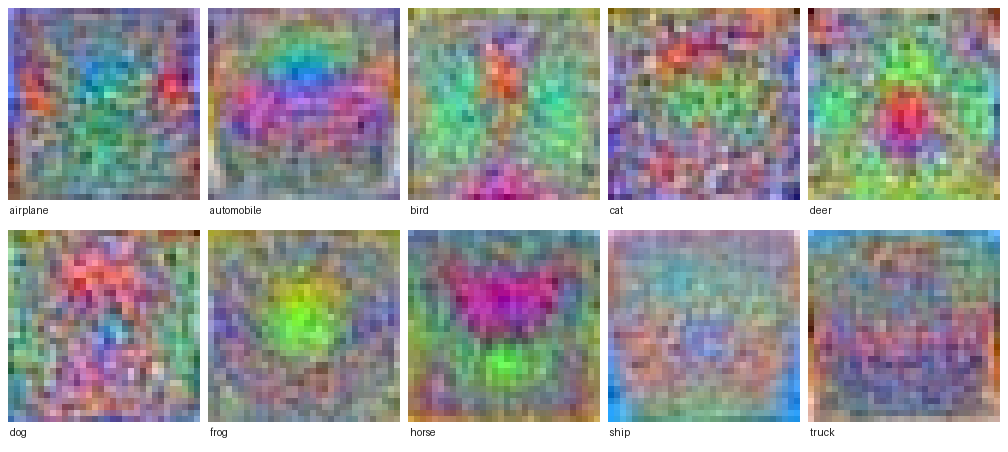
None of these are sharp pictures, exactly as described above: each is a blurry average of thousands of training photos. But they still show recognizable structure. “Ship” has blue along the bottom (water) and “airplane” has blue along the top (sky). “Frog” has a green blob in the middle. “Automobile” shows a reddish car-body shape. Up close, “horse” looks like a two-headed animal: the training setthe images the model learns from. has horses facing both left and right, and a single template has to average them into one smear.

But here’s the limitation: a linear classifier uses just one set of weights per class, one weight for each pixel value, so it can only look for one pattern per class. A single dog template won’t match every dog, and this is where the seven challenges from Part 2 come back. A dog seen from the side, a dog far away and tiny, a dog in shadow, a Chihuahua versus a Great Dane: each produces a different grid of numbers, and a single template, being the average of all of them, matches each one only poorly.

An obvious response: fine, just use more templates. One for “side view dog,” one for “front view dog,” one for “small dog,” one for “dog in shadow.” That does help, up to a point. But it runs into two walls.

The first is a combinatorial explosion (the number of cases blows up as the challenges combine). You don’t need one extra template per challenge; you need one for every combination of them: small-and-dark-and-side-view dog, large-and-bright-and-front-view dog, and so on across all seven axes at once. That is not seven or seventy templates, it is millions, and you would need enough labeled photos to learn each one.

The second is that two of the challenges don’t yield to more templates at all. Background clutter is different in every photo, so a template, which has one fixed value per pixel position, has no consistent background it can match. And a dog can be occluded (partly hidden) in endless ways, so there’s no single “occluded dog” to memorize.

That single-template limit is why a linear classifier tends to do better on simple, consistent images than on messy real-world ones.

The fix the field actually adopted is not more whole-dog templates. It’s to learn small, reusable pattern detectors, things like edges, textures, and parts, that combine to recognize a dog in any pose. Reusable detectors like these are what neural networks (Part 9) are built on. Convolutional networks (Part 12 onward) go one step further and reuse the same detector at every position, so a single “ear” detector helps no matter where the ear sits. That is where the rest of this series is headed.

The Missing Piece: How the Weights Get Learned

But before we fix that limitation, we need to understand the learning process itself. How does the computer know which direction to adjust the weights? How much should it adjust? What’s the measure of “wrongness” that guides the learning?

That’s loss functions (a number measuring how wrong the scores are) and gradient descent (the method for adjusting the weights to reduce that number): the next two posts.

For now, just understand this: a linear classifier scores images with a weighted sum of pixels, picks the highest score, and learns those weights from training data.