Paper #1, Part 9: Neurons and Networks (Stacking Simple Decisions Into Something Smart)
A single linear classifier is rigid. But what if you stack multiple layers, each adding non-linearity? That gives you a neural network.
Where we are: we have built and trained a single linear classifier (Parts 5 to 8). Now we stack many simple units into a neural network that can learn far more complex patterns.
From Part 5: a linear classifier computes a weighted sum of pixels and picks the highest score.
The problem: one linear layer can only learn linear decision boundaries. If your classes aren’t linearly separable (and most real-world data isn’t), no straight-line boundary can tell them apart.
The solution: change the function. Back in Part 1 we said the function is ours to change however we like, as long as the change makes it better at predicting. Turning a straight-line function into a curved one is exactly that kind of change. The usual way to do it is a neural network: stack multiple layers, add a non-linear step between them, and the function can bend into curved boundaries and more complex patterns. That non-linear step can take a few forms, which we get to below.
The Neuron
A neuron is the basic unit. It takes inputs, multiplies them by weights, adds a bias (a constant that shifts the result up or down, the + b in y = mx + b), and applies an activation function.
output = activation( (w1*x1 + w2*x2 + ... + bias) )That inner sum (w1*x1 + w2*x2 + ... + bias) is the same “score” a linear classifier produced in Part 5: weights times inputs, plus a bias. It’s called the neuron’s pre-activation, and it’s what gets passed to the activation function.
The activation function is non-linear, meaning its output doesn’t move in simple proportion to its input; it can bend or flatten instead of following a straight line. Common ones:
ReLU (Rectified Linear Unit):
f(x) = max(0, x)If the sum is positive, pass it through. If negative, zero it out. It’s one of the simplest activation functions there is, and per the CS231n notes, the most common choice in networks when those notes were written.
Sigmoid:
f(x) = 1 / (1 + e^(-x))Squashes any input to a value between 0 and 1. It was common in earlier networks, before ReLU became the default.
Tanh:
f(x) = (e^x - e^(-x)) / (e^x + e^(-x))Squashes to between -1 and 1. A scaled, shifted version of the sigmoid, and like sigmoid a common choice before ReLU; it was often preferred because its outputs are centered on zero rather than always positive.
Which activation a layer uses is a hyperparameter, a choice you make before training (Part 7), just like the number of layers, not something the network learns on its own.
Why it matters: without the activation function, stacking linear layers just gives you another linear layer (stacking straight-line steps only ever gives you another straight-line step). The activation function breaks this chain and lets the network learn curved, non-linear patterns.
Stacking Layers
The idea is to stack multiple layers, each with its own weights and activation:
Input (pixels)
  → [Linear layer 1] → [ReLU]
  → [Linear layer 2] → [ReLU]
  → [Linear layer 3] → [ReLU]
  → [Linear layer 4 - final scores]
Each layer transforms the output of the layer before it, and the network can build up features in stages: early layers picking up low-level patterns like edges, later ones combining those into bigger pieces, and still later ones responding to higher-level concepts. This progression from simple edges to whole objects is something the convolutional networks in Parts 12 to 14 are built for; plain stacked layers like these manage it only as far as the data and training allow.
The final layer then uses those built-up features to make the actual decision, like cat versus dog.
Why This Works
With one linear layer, you can only draw straight lines to separate classes. Add a non-linear activation and the boundary can bend into curves; add more neurons and more layers, and it can take on more and more intricate shapes.
The more neurons and layers you add, whether as wider layers (more neurons) or deeper stacks (more layers), the more complex the boundaries the network can represent. It also means more numbers to learn (the weights and biases) and more risk of overfitting: the network memorizing quirks of the training data instead of the general pattern (more on that in Part 11).
Width and Depth
Here is that stacking diagram again:
Input (pixels)
  → [Linear layer 1] → [ReLU]
  → [Linear layer 2] → [ReLU]
  → [Linear layer 3] → [ReLU]
  → [Linear layer 4 - final scores]
Chaining one layer into the next like this, each working on the output of the one before it, is what depth means. That network is four layers deep. (The [ReLU] boxes aren’t extra layers. Each just applies the activation to the linear layer right before it, the same activation built into every neuron. A linear box and its ReLU together make one layer.)
What the diagram hides is what sits inside each box. A box labeled “Linear layer” is actually a column of neurons, and how many neurons fill that column is the layer’s width. Here is the whole picture at three zoom levels: a single neuron, then one layer, then several layers chained.
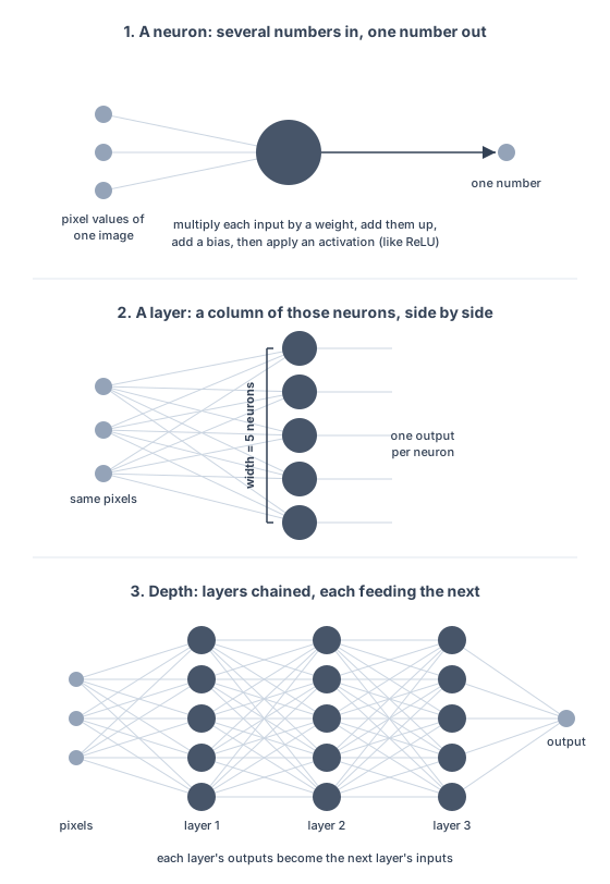
So they are two separate choices. Depth is how many layers you chain one after another; width is how many neurons are packed inside a single layer. A network can be deep and narrow, shallow and wide, or anything in between.
The widths don’t even have to match from layer to layer. Each hidden layer’s width is its own choice, another hyperparameter you set before training (like the depth and the activation function), so one layer can be wider or narrower than the one before it. The figure above drew five neurons in every layer just to keep the panels tidy; a real network’s layers are usually different sizes. The one width that isn’t free is the last layer’s: it’s fixed by the task, with one output neuron per possible answer (in this case three, for cat/dog/bird).
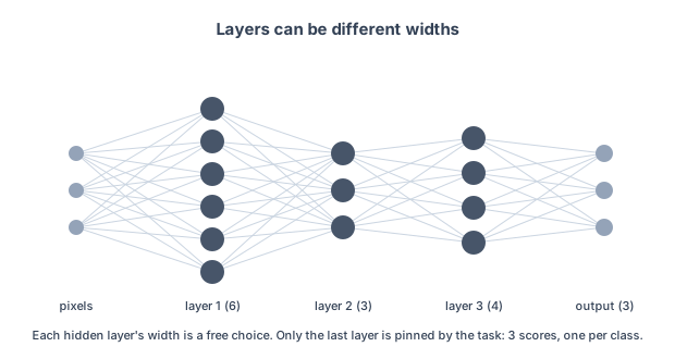
This is also where a model’s huge weight count comes from. Every line in the figure is a separate weight, and each neuron has its own weight for every input, so a single pixel is multiplied by a different weight in each neuron. If an image is 3,072 numbers (the 32×32×3 from Part 5) and a layer has 100 neurons, that one layer holds 100 × 3,072 = 307,200 weights, plus 100 biases (one per neuron). Stack several wide layers and the total climbs into the millions or billions. Those learned numbers, the weights and biases together, are what people call a model’s parameters. When a headline says a new model has 500 billion parameters, it means 500 billion individual numbers the model adjusted during training.
The theorem in the next section is about the shallow-and-wide extreme: a single hidden layer, made wide enough.
The Universal Approximation Theorem
There’s a mathematical result, the Universal Approximation Theorem, with a surprising message. Take a network with a single layer of neurons in the middle, between the input and the final answer; that middle layer is called a hidden layer (hidden because you never see its values directly, they’re an internal step). Give it enough neurons, and it can mimic almost any function you could draw, to as much accuracy as you want.
That is a sweeping claim, and it comes with a catch. The theorem says such a network can represent the function, not that it will learn it. Those are two different things:
- Represent: somewhere among all the possible settings of the network’s weights (its millions of knobs), a setting exists that matches the target function.
- Learn: training, starting from random weights and nudging them based on the data, can actually arrive at that setting.
Think of a safe. The theorem guarantees the safe has a combination that opens it. It says nothing about whether you can find that combination, and finding it can fail even though it exists:
- Gradient descent (Part 7) walks downhill from wherever it happened to start, and it can settle into a mediocre valley without ever reaching the best setting.
- You might not have enough data to tell which weight settings are the right ones.
- “Enough neurons” could be an impractically huge number.
So the theorem promises only that a good setting exists. Whether training reaches it, with a sane number of neurons and the data you have, is a separate question.
And “one hidden layer is enough in principle” doesn’t make depth pointless. In practice, stacking more layers usually captures complex patterns more efficiently, with fewer neurons, than one very wide layer, and the way the network is arranged (its architecture) strongly affects what it actually learns.
What’s Next
We now have the building block: neurons with non-linear activations, stacked into layers.
But we still need to prepare the data properly. Feeding raw pixel values (0-255) directly into a network can cause training problems. That’s data preprocessing, which is Part 10.