Paper #1, Part 10: Garbage In, Garbage Out (Why Data Prep Matters)

Where we are: we can build and train neural networks (Part 9). Before they work well, though, the data you feed them has to be prepared properly.

Neural networks are sensitive to the scale of their inputs, and pixels come in a wide range: 0 to 255.

Recall from Part 8 that a weight’s adjustment is its blame times the input feeding it, so, with the same blame, a bigger input means a bigger adjustment. Raw pixels run all the way up to 255, big enough to make those adjustments large and erratic, so training can be unstable and slow.

The fix: normalize the inputs, shrinking them to a small, consistent range.

Normalization

The simplest approach: divide every pixel by 255, so the values run from 0 to 1 instead of 0 to 255.

normalized_pixel = raw_pixel / 255

Now every input is between 0 and 1 instead of up to 255: small, comparable numbers for the network to work with.

A more thorough approach is standardization. Dividing by 255 only shrinks the numbers; standardization also re-centers them around zero.

standardized_value = (raw_value - average) / standard_deviation

Subtract the average (the mean) and divide by the standard deviation (how far a typical value sits from the average), both measured on your training data and then applied unchanged to any new data. This puts the values around zero and on a comparable scale, which makes training go more smoothly (the next section shows why).

This is the same move as curving a test: subtract the class average from your score, then divide by how spread out the scores were. A raw 82 tells you little on its own, but “1.5 standard deviations above average” is comparable across any class, however hard it was graded. Standardization does that to every feature.

Why This Matters

Pixels all live on the same 0-to-255 scale, so a single division by 255 shrinks them into a small range together. It gets trickier when a model’s features are on different scales from each other, because then no single divisor works for all of them.

Say a model predicts a house’s value, and one house has two features:

• Bedrooms: 4
• Square footage: 2500

From Part 8, the gradientthe slope of the loss for each weight: which way, and how steeply. for a weight (the number that sets how far it moves) is the blame arriving at it (its share of the error) times the feature it multiplies. With the same blame, 1, reaching both weightsthe numbers inside the model that it adjusts as it learns.:

bedrooms weight's gradient       = 1 × 4    = 4
square footage weight's gradient = 1 × 2500 = 2500

The square-footage weight’s gradient is over 600 times bigger, not because square footage matters more, but only because it is counted in bigger numbers than bedrooms. Each step moves a weight by the learning ratehow big a step to take on each weight update. times its gradient, so with one learning rate for both, the square-footage weight lurches while the bedrooms weight barely moves. One rate can’t serve both, so training stalls or thrashes.

Standardization (from the start of the post) fixes this. For each feature, it measures that feature’s own average and standard deviation. Then it subtracts the average and divides by the standard deviation.

Suppose bedrooms average 3, with most houses within about 1 of that (a standard deviation of 1), and square footage averages 2000, with most homes within about 1000 of that:

bedrooms standardized       = (4 - 3) / 1          = 1
square footage standardized = (2500 - 2000) / 1000 = 0.5

Both now sit on the same small scale, comparable in size (1 and 0.5) instead of wildly apart (4 and 2500). That is by design, not coincidence: standardization expresses every feature as how far a value sits from its own average, measured in standard deviations, so features that started in different units come out comparable in size. Dividing everything by one number, the way we divided pixels by 255, wouldn’t do this, because bedrooms and square footage are on different scales; each needs its own average and standard deviation. Now the gradients are comparable:

bedrooms weight's gradient       = 1 × 1   = 1
square footage weight's gradient = 1 × 0.5 = 0.5

so the two weights move at similar rates, and a single learning rate works for both. That is the point of normalizing: put every input on a comparable scale, so no weight is updated wildly harder than another just because its input happened to be bigger.

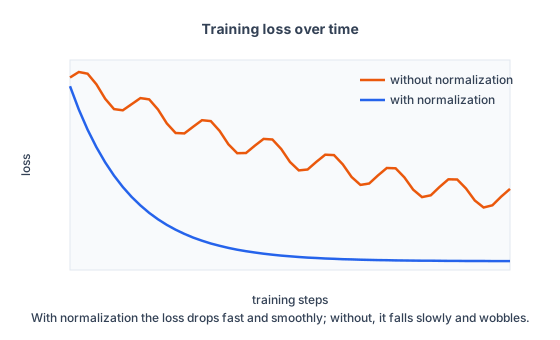
In practice, normalizing usually makes the lossa single number measuring how wrong the current guesses are. drop faster and more smoothly; without it, the loss falls slowly and wobbles, because no single learning rate fits both the large and small gradients.

And none of this is specific to house prices or pixels: any time a model’s features are on very different scales, standardizing them first keeps the big-numbered ones from dominating. Features already on a small, similar scale need it less.

What’s Next

Now we have networks with layers and activations, and inputs that are properly scaled.

The next challenge is overfitting: a network can end up memorizing its training examples instead of learning the general pattern, so it does well on data it has seen and poorly on data it hasn’t. Part 11 covers why that happens and how to curb it, with regularization.