Paper #1, Part 11: Memorizing vs. Learning (Overfitting and Regularization)

Where we are: we can train a network on well-prepared data (Parts 9 and 10). But a network can memorize instead of learn, and this post is how to tell the difference and prevent it.

You build a neural network. Train it on your training setthe images the model learns from.. It achieves 99% accuracy.

You try it on data it hasn’t seen. 60% accuracy.

What happened? Overfitting.

The network memorized the training data instead of learning generalizable patterns. It latched onto quirks specific to your training set, behaving as if it had memorized rules like “if pixel 47 is exactly 128 and pixel 92 is exactly 200, it’s a cat.” Those exact combinations hold on the training images but fall apart on anything new.

Training vs. Validation Accuracy

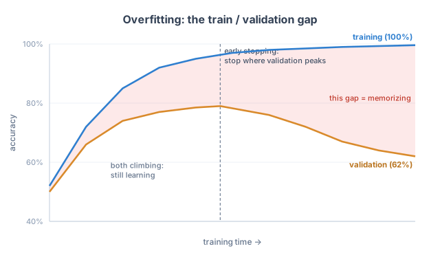
The gap between training accuracy and accuracy on a validation setheld-out images used to compare designs and tune settings. (data held out from training to check progress, from Part 4) is the main sign of overfitting:

• Small gap (90% train, 88% validation): Good generalization. The network learned actual patterns.
• Large gap (99% train, 60% validation): Severe overfitting. The network memorized.

The bigger your network and the smaller your dataset, the more prone to overfitting it tends to be. A network with a million parameters can memorize a dataset of 1,000 images with ease.

Regularization: Fighting Overfitting

The common thread across the techniques below is to hold the network back: make it a little harder to fit the training data exactly, so the network is nudged toward the broad pattern instead of the fine-grained quirks. Each does this in a different way.

L2 Regularization (Weight Decay)

Memorizing quirks takes sharp, extreme responses to tiny differences between images, and sharp responses require large weightsthe numbers inside the model that it adjusts as it learns. (a big weight lets a single input swing the output hard). So one way to discourage memorizing is to discourage large weights. L2 regularization does exactly that, by adding a penalty to the lossa single number measuring how wrong the current guesses are. that grows with the size of the weights:

total_loss = classification_loss + λ * (sum of squared weights)

Here λ (the Greek letter lambda) is a number you choose, the penalty strength. It makes the optimizer balance two goals: fit the training data (the first term) and keep the weights small (the second). A bigger λ pulls harder toward small weights; a smaller one lets the network fit the data more freely. The network settles on the smallest weights that still fit the data well, the ones that capture the general pattern rather than the large ones that fit quirks.

Why squared, rather than just adding up the weights? A raw sum doesn’t measure size: positive and negative weights cancel (a +1000 and a -1000 add to zero), and the optimizer could even shrink the penalty by driving weights very negative. To penalize size, you have to drop the sign, either by squaring or by taking the absolute value. Squaring (L2) is the common default because it grows fast, so it comes down hardest on the few largest weights, exactly the ones that let a network overfit. The absolute-value version, L1 regularization, is the main alternative; it tends to push weights all the way to zero rather than just shrinking them.

Dropout

During training, randomly “drop” (set to zero) a fraction of neuronsone unit that weights its inputs, adds them up, and applies an activation.. If 50% dropout is used, each neuron has a 50% chance of being zeroed out on each forward pass.

Why? Because any neuron might be dropped on a given pass, the network can’t rely on any single one to carry critical information. The work has to be spread across many neurons, so no fragile, one-off pattern can take hold.

It’s like a basketball team that benches a different random player every practice. Because no one knows who will sit out, everyone has to learn every position, and the team stops leaning on any single star. A network trained with dropout spreads its knowledge the same way.

At test time, every neuron stays on, and nothing special happens. Modern frameworks handle the bookkeeping during training instead: when some neurons are dropped, the outputs of the ones that remain are scaled up to compensate, so the totals line up once all the neurons are active at test time.

Dropout is simple and widely used.

Early Stopping

Monitor the validation accuracy as training goes. When it stops improving for a while, stop, even if training accuracy could still climb. (You wait rather than stopping at the first dip, since validation accuracy naturally wobbles.)

Left training too long, a network starts fitting the training set’s quirks after it has already learned the general pattern; stopping early avoids that.

More (or Augmented) Data

The most direct cure for overfitting is simply more training data: quirks are harder to memorize across a larger, more varied set. When you can’t gather more, you can expand it with data augmentation: making modified copies of the examples you already have. For images, small flips, crops, and color shifts turn one example into many, all still clearly the same class.

The Balance

Regularization reduces overfitting, but too much of it underfits: the network is so constrained it can’t learn the task at all.

Getting the balance right means tuning several things:

• Penalty strength (λ)
• Dropout rate
• Network size (a bigger network needs more data to avoid overfitting)
• Amount of training

This is where hyperparametera setting you choose before training, not learned from data. tuning comes in: trying different settings and keeping what generalizes best. You judge “generalizes best” on the validation set; the test setheld-out images used once, at the end, for the final score. stays untouched until the very end, as a final, unbiased check (Part 4), since tuning against the validation set can slowly overfit it too.

What’s Next

We’ve covered the fundamentals of neural networks: architecture, activation functionsa simple bend applied to a neuron's output, like ReLU., data preparation, and preventing overfitting.

Now it’s time to move from general neural networks to a specific, powerful architecture designed for images: convolutional neural networks. Part 12 introduces convolutions, the core idea behind modern computer vision.