Paper #1, Part 8: Backpropagation (How Blame Gets Passed Backward)

Where we are: gradient descent improves the weights by stepping downhill (Part 7), but every step needs the slope for each weight. This post is how those slopes get computed.

From Part 7: gradient descentrepeatedly nudge the weights downhill to shrink the loss. adjusts weightsthe numbers inside the model that it adjusts as it learns. using gradientsthe slope of the loss for each weight: which way, and how steeply., the slope of the lossa single number measuring how wrong the current guesses are. for each weight. So the job now is to compute those slopes. In calculus terms, that might sound easy (just differentiate the loss), so why does it need a special algorithm at all?

For a simple function, it is easy. Take a loss like:

loss = (w - 5)² + (z + 2)⁴ + (a - 3)²

Each weight sits in its own separate term. The slope for w is just 2(w - 5), from the first term; the slope for z is 4(z + 2)³, from the second. Every weight is independent, and computing all their slopes is quick. If a network’s loss looked like this, we wouldn’t need anything clever.

But a network’s loss isn’t a tidy sum like that. Its weights are all tangled together: nudge one weight early on, and its effect passes through every layer after it before reaching the loss.

Picture a short chain, where the input is multiplied by one weight, then that result by the next weight, then that by the next. Starting from an input of 2:

2  →  ×3  →  6  →  ×4  →  24  →  ×5  →  120

Nudge that first weight from 3 to 3.1, and the 6 becomes 6.2, the 24 becomes 24.8, and the final 120 becomes 124. How much that nudge moved the answer depended on the weights the change flowed through: make the ×4 or the ×5 bigger, and the same nudge would move the answer more. That sensitivity, how much the answer moves when you nudge the weight, is what the weight’s slope measures, and here it isn’t the weight’s own private number; it’s tangled with every weight after it. In the tidy sum earlier, each weight’s slope came from its own separate term alone. Here it doesn’t.

You can still work out every slope with calculus. The catch is that doing it one weight at a time repeats a huge amount of the same work, since all those weights share the same path forward to the loss. For a network with millions of weights, that’s hopeless.

Backpropagation is the shortcut. It computes the exact same slopes calculus would, just far faster: all of them in one sweep backward through the network, doing each shared piece of work once instead of millions of times. That matches the hunch that a computer should just be able to take the derivativethe slope of a function: how its output changes as its input changes.: it can, and backpropagation is the efficient way it does it. The rest of this post is how, and it comes down to an idea from calculus called “the chain rule”.

The Chain Rule

Our goal hasn’t changed: we still want to know how much y (our loss) changes when we nudge x (our weight). (That change in y with respect to x is referred to as dy/dx, and it’s the same slope idea from before.) The d just means “a tiny change in,” so dy/dx is a tiny change in y divided by the tiny change in x that caused it.

In the separable example from the opening, that was easy: every term stood on its own, so each slope was a one-step calculation. A step closer to how machine learning actually works is a nested equation, one equation tucked inside another. For example:

y     = inner²
inner = x³ + 5x

y isn’t written directly in terms of x. It’s written in terms of inner, and inner is written in terms of x, one equation sitting inside the other. (A neural network, the kind of model behind tools like ChatGPT, is this same nesting taken much further: layer inside layer inside layer. It’s where this series is headed next.)

The nesting is what gets in the way of our goal: x is buried inside inner, which is buried inside the squaring, so we can’t read off how y responds to x in a single move.

The chain rule resolves this by going through the middle. To get how y changes as x changes, you multiply two simpler rates of change:

• how much y changes as inner changes, and
• how much inner changes as x changes.

For our example:

• y = inner², so y changes at a rate of 2 × inner as inner changes, which is 2(x³ + 5x).
• inner = x³ + 5x, so inner changes at a rate of 3x² + 5 as x changes.

Multiply them:

dy/dx = 2(x³ + 5x) × (3x² + 5)

The nesting is handled by chaining two local rates of change through the middle.

The rates above (why inner² changes at 2 × inner, and x³ + 5x at 3x² + 5) come from a part of calculus called derivatives. For a quick refresher on the specific rule used here, Math Is Fun has a short page on the power rule. For a deeper, visual explanation of what derivatives are, 3Blue1Brown’s Essence of Calculus is a great place to start.

The Assembly Line Metaphor

Imagine a factory assembly line. A component moves through several stations:

Input → [Station A] → [Station B] → [Station C] → Output

At each station, workers add value (or subtract it). The final output depends on what happened at every station.

Now imagine the output is wrong. Quality control finds a defect. Who’s to blame?

The defect isn’t the last station’s fault alone. Blame propagates backward through the line:

• “Why is the output bad? Because Station C did bad work, or because the input to Station C was bad.”
• “Why was the input to Station C bad? Because Station B did bad work.”
• “Why was Station B’s output bad? Because Station A did bad work, or because the original input was bad.”

Each station needs to know: “How much of the final defect is my fault?”

Backpropagation does exactly this for a neural network: it works out how much each weight is to blame for the loss, passing blame backward through the function.

How Backpropagation Works

A linear classifierscores an image with a weighted sum of its pixel values. (such as our cat / dog / bird image classifier) is just one step: for each class (i.e. “cat”, “dog”, “bird”), multiply every pixel by that class’s weight for that pixel, add the results into a single score, then add a “bias” for that class on top. (In the school-algebra line y = mx + b, the biasa constant added to a score; it shifts the result up or down. is the + b, a constant that shifts the score up or down regardless of the pixels; the weights are the m. It was introduced in Part 5.)

Then compute the loss:

pixels → [ multiply by weights, add biases ] → scores → [ compute loss ] → loss

Those two bracketed steps are the “stations” from the last section. The first takes the pixels in and puts out the three class scores; the second takes those scores in and puts out the loss (how wrong the guess was). The weights live inside that first station, so that’s where the blame has to end up.

Each training step has two passes, and backpropagation is the second one.

Forward pass: the ordinary run from Parts 5 and 6, feeding the input through the function to produce the scores and then the loss. Along the way, save the intermediate results at each station.

Backward pass (this is backpropagation): starting from the loss, work out how much the loss would change if each station’s output changed a little. That number is the station’s “blame.” Using the values the forward pass just saved, apply the chain rule to propagate it backward through each layer.

This forward-then-backward pair runs on every training step. The weights change after each step, so the next step reruns the forward pass and recomputes fresh intermediate results; they are never captured once and reused.

At each station, blame flows backward by multiplying two numbers:

• Incoming blame: how much the final loss changes when my output changes. For example, if my output changes by 2 and the loss changes by 5, the incoming blame is 5 ÷ 2 = 2.5.
• My local effect: how much my output changes when my input changes. For example, if my input changes by 5 and my output changes by 6, the local effect is 6 ÷ 5 = 1.2.
• Blame I pass back to my input: 2.5 × 1.2 = 3.0.

By the time you reach the weights, you know exactly how much each weight affects the final loss.

A Worked Example: A Confidently Wrong Guess

Take the confidently-wrong case from Part 6: the true label is cat, but the scores come out cat 3, dog 10, bird 1. The classifier is sure it’s a dog. Let’s watch the blame flow backward.

Turn the scores into probabilities (softmaxturns raw scores into probabilities that add up to 1., from Part 6):

P(cat)  = 0.0009   (should be 1)
P(dog)  = 0.999    (should be 0)
P(bird) = 0.0001   (should be 0)

The loss is high, because the correct label got almost none of the probability.

Blame on each score. For this softmax-and-loss setup, the blame on each score works out to something remarkably simple: the probability the model gave, minus the probability it should have given (1 for the correct label, 0 for the rest).

blame on cat's score  = 0.0009 - 1 = -0.9991
blame on dog's score  = 0.999  - 0 =  0.999
blame on bird's score = 0.0001 - 0 =  0.0001

Cat’s blame is strongly negative, meaning its score is far too low and we should push it up. Dog’s is strongly positive, meaning its score is far too high and we should push it down. Bird’s is tiny, meaning its score is about right and we can leave it alone. Exactly the correction a confidently-wrong guess deserves.

One step further back, to a weight. Those score blames are now the incoming blame for the next station back. Each score is a weighted sum of the pixels, so a weight’s local effect on its score is just the pixel it multiplies. Multiply the two, exactly like the last section. Take one of dog’s weights sitting on a bright pixel in this image, value 200: its incoming blame is dog’s score blame (0.999), and its local effect is that pixel (200), so:

blame on that dog weight = 0.999 × 200 ≈ 200

The blame is positive, so gradient descent lowers that weight, and dog scores a little lower on images with that pixel next time. Every dog weight on a pixel that lit up this image gets the same downward push.

That’s the whole backward pass: blame started at the loss, flowed to the three scores, then on to the weights, each step just simple arithmetic.

Why This Is Fast

If you estimated the gradients numerically (nudge each weight a tiny bit, rerun, and see how much the loss changed), you’d need to:

1. Change weight #1 by 0.0001, run the full forward pass, measure the loss change → gradient for weight #1
2. Change weight #2 by 0.0001, run the full forward pass, measure the loss change → gradient for weight #2
3. Repeat for all 3,000 weights

That’s 3,000 full forward passes, one for every weight, and real networks have millions of them.

Backpropagation does it in one forward pass and one backward pass, no matter how many weights you have.

The chain rule means: once you’ve computed blame at one layer, you can quickly compute blame at the previous layer. You multiply by the chain rule factor and move on.

What Backpropagation Comes Down To

Backpropagation isn’t magic. It’s just:

1. The chain rule from calculus
2. Applied step by step to a function built by nesting, one step inside another
3. In reverse order (backward)

Each of those nested steps is a layer (like inner = x³ + 5x, then the squaring after it). What makes this work is that each layer only needs to know its own local behavior, how its output depends on its input. It doesn’t need to understand the whole function. The chain rule carries each layer’s local information backward and combines it into the slope for every weight.

This efficiency is what makes training large networks possible at all: each layer contributes just a local calculation, and backpropagation chains them together into the slope for every weight, however many layers and weights there are.

What’s Next

Now we have:

• A way to score images (linear classifiers)
• A way to measure wrongness (loss functionsthe rule that turns the guesses and answers into the loss number.)
• A way to find gradients (backpropagation)
• A way to improve weights (gradient descent)

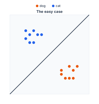
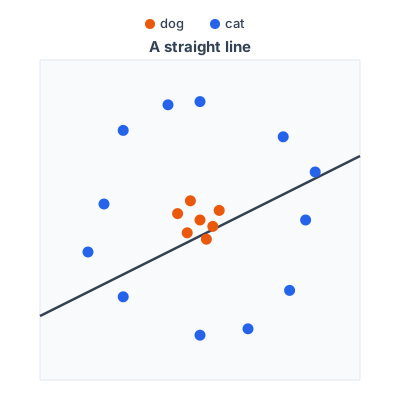
But our classifier is still a single weighted sum, and that has a hard limit. Picture each image as a dot on a graph, with cats in one area and dogs in another. Classifying them means drawing a boundary that puts every dog on one side and every cat on the other.

The easiest case is when the two groups are cleanly split: all the cats over here, all the dogs over there. Then a single straight line does the job, and a weighted sum can draw that straight line.

Real data is messier. Here the dogs cluster in the middle and the cats surround them, and no straight line can separate the two: wherever you draw it, some dogs or some cats end up on the wrong side.

Which is why we need a curve, not a straight line. A curved boundary can wrap around the dog cluster, putting every dog on the inside and every cat on the outside.

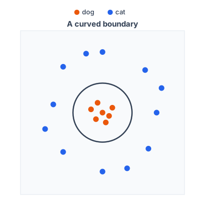
But a plain weighted sum can only ever draw straight lines. To bend the boundary, you keep the weighted sums and add a non-linear step after each one; stacking many such layers is what lets the boundary curve. That’s a neural network, and it’s where the series goes next.