Paper #1, Part 7: Learning by Trial and Error (Gradient Descent)

Where we are: we can score an image (Part 5) and measure how wrong the score is (Part 6). Now we use that measure to adjust the weights and make the scores better.

We have a loss functionthe rule that turns the guesses and answers into the loss number. that measures how wrong we are. We want to make that number smaller.

How?

Gradient descent is the algorithm that adjusts the weightsthe numbers inside the model that it adjusts as it learns. to reduce lossa single number measuring how wrong the current guesses are.. It’s the core idea behind how most neural networks are trained and improved, including the ones in this series, though other kinds of machine learning models (like decision trees) are trained in different ways.

The Downhill Metaphor

Imagine you’re on a foggy mountain. You can’t see the valley, but you can feel the slope of the ground beneath your feet. This landscape can have many separate valleys, and in the fog you only ever feel the slope right under your feet, not the whole terrain.

Your goal: reach the lowest point.

Strategy: repeatedly take a step downhill. Feel the slope, step in the direction that goes down, repeat.

If all goes well, each step takes you a little lower, and eventually you settle into a valley.

That’s gradient descent.

Replace “mountain slope” with “loss function” and “step downhill” with “adjust weights” and you’ve got the algorithm.

How It Works: The Gradient

In mathematics, the gradient of a function points in the direction of steepest increase, the steepest uphill direction. To go downhill, you head the opposite way.

At a single spot, the steepness isn’t one number. It depends on which way you face. Step north and the ground might barely rise; step east and it might climb sharply. So a point has a slope for every direction you could move, and the gradient bundles those together to point at the single steepest one.

A real mountain has two directions to weigh (north-south and east-west). A loss function has thousands, one for each weight. For each weight you measure its own slope: if you nudge this weight up a little, does the loss rise or fall, and by how much? (A slope like this is what calculus calls a derivative; the slope for one weight among many is a partial derivative.) Those thousands of slopes together are the gradient.

Then you adjust each weight a tiny bit in the direction that reduces loss.

Repeat this thousands of times, and the weights gradually improve, as long as each step is the right size.

Learning Rate: Step Size

How much should you adjust each weight?

If you take huge steps, you might overshoot the valley and end up on the other side, higher than before. In loss terms, the loss goes up instead of down: the new weights are worse than the old ones.

If you take tiny steps, you’re safe but it takes forever to reach the bottom.

The learning rate is the step size. You don’t guess it blindly; people usually start from common defaults like 0.01 or 0.001 and adjust from there.

new_weight = old_weight - learning_rate * gradient

If the learning rate is too high, training is unstable: the loss bounces around, and in the worst case it grows without bound instead of settling, a failure called divergence.

If the learning rate is too low, training is slow but stable.

In most practical guides, the learning rate is one of the first hyperparametersa setting you choose before training, not learned from data. (settings you pick before training, unlike the weights the model learns on its own) that people tune.

A Concrete Example

Let’s say we have one weight w and a simple loss function:

loss = (w - 5)²

The minimum is at w = 5 (loss = 0).

This (w - 5)² isn’t one of the loss functions from Part 6 (hinge or softmaxturns raw scores into probabilities that add up to 1. loss). It’s a stand-in, chosen to be as simple as possible: one weight instead of thousands, and an obvious lowest point, so we can run gradient descent by hand and watch it converge. Part 6’s losses are functions of thousands of weights at once, which you can’t step through on paper.

The gradient at any point w is:

gradient = 2(w - 5)

Let’s start with w = 0 and learning rate = 0.1:

Iteration 1:

• current loss = (0 - 5)² = 25
• gradient = 2(0 - 5) = -10
• new_w = 0 - 0.1 * (-10) = 0 + 1 = 1

Iteration 2:

• current loss = (1 - 5)² = 16
• gradient = 2(1 - 5) = -8
• new_w = 1 - 0.1 * (-8) = 1 + 0.8 = 1.8

Iteration 3:

• current loss = (1.8 - 5)² = 10.24
• gradient = 2(1.8 - 5) = -6.4
• new_w = 1.8 - 0.1 * (-6.4) = 1.8 + 0.64 = 2.44

The loss is decreasing: 25 → 16 → 10.24. We’re moving downhill. After many iterations, w converges to 5 and loss approaches 0.

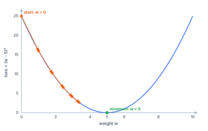
Each orange dot is one iteration. The steps shrink as you near the bottom: far from the minimum the slope is steep, so the step is big; close to it the slope is gentle, so the step is small. That’s why w eases into the minimum instead of shooting past it.

Why This Works

One way to look at training is as a search for the weight values that make the loss as small as possible. Gradient descent is the search strategy, and it works because:

1. Local information guides global movement: You don’t need to see the whole valley. Just look at the slope beneath your feet.

2. Repeated small steps add up: Even if each step is small, thousands of steps can cover a lot of ground, though how fast you get there depends on the learning rate and the shape of the loss.

3. Automatic feedback: The loss number tells you how wrong you currently are. With a good learning rate it drops every step; if it starts rising, that’s the sign the learning rate is too high.

4. Generalizes to any number of weights: The same algorithm works whether you have one weight or a million. More advanced variants of it train today’s large language models, which have hundreds of billions of weights.

The catch: gradient descent finds local minima, not necessarily the global minimum. On a mountainous landscape, you might settle into a valley when a deeper valley exists elsewhere. This sounds like a serious problem, but in practice, with large networks and the more advanced variants of gradient descent used today, training usually reaches a solution that works well, even if it isn’t the single lowest point. Finding the exact global minimum turns out not to be necessary.

What’s Next

Every step of gradient descent needs the gradient: the slope for each weight. The update itself, taking a small step downhill, is the same whether you have one weight or a billion. But it assumes the slopes are already in hand.

Getting that slope was easy in the one-weight example above: using high-school calculus, it’s just the derivative of (w - 5)², which comes out to 2(w - 5). With billions of weights, it gets much more complicated. The next post shows why, and how it’s solved, with an algorithm called backpropagation.