Paper #1, Part 6: How Does the Computer Know It's Wrong? Loss Functions

Where we are: we have a linear classifier that gives each image a score (Part 5). To make those scores better, we first need to measure how wrong they are.

From Part 5: a linear classifierscores an image with a weighted sum of its pixel values. computes scores for each label and picks the highest one.

Now, if the highest score is the wrong label, how wrong is it? And how do you tell the computer to improve?

The answer is loss functions.

Wrongness as a Number

A naive approach: a prediction is either right or wrong. Binary. You get 1 point or 0 points. This seems logical, and it’s fine for reporting a final accuracy score, but it’s too coarse to guide learning: it can only tell the computer whether it was right or wrong, not how to improve.

Imagine three scenarios. In each, the correct label is “cat,” and the classifier has produced a score for every label.

Scenario A (a close call):

• cat: 10
• dog: 9.5
• bird: 8

The classifier picks “cat” (correct), but dog was nearly as high. This feels uncertain.

Scenario B (a confident call):

• cat: 100
• dog: 1
• bird: 0.5

The classifier picks “cat” (correct), and the others are far behind. This feels confident.

Scenario C (a mistake):

• cat: 3
• dog: 10
• bird: 1

The classifier picks “dog” (wrong). Cat, the correct answer, scored well below it.

If you only count right or wrong, A and B both score 1 (correct) and C scores 0 (wrong). That misses two things: it can’t tell the confident B apart from the shaky A, and it can’t say whether C was a near miss or a wild miss.

A loss function measures not just whether the guess was right, but how right, or how wrong. We’ll compute two common loss functions, hinge loss and softmax loss, on these same three scenarios.

Hinge Loss

Here’s one approach called hinge loss. It’s the loss function used by Support Vector Machines (SVMs), a traditional type of classifier that predates deep learning.

For each scenario, take two numbers: the correct label’s score (correct_score) and the highest wrong label’s score (wrong_score). (The standard multiclass version adds up a penalty across every wrong label; we use just the single highest wrong score here to keep it simple.) The loss is:

loss = max(0, 1 + wrong_score - correct_score)

Here max(a, b) just means “take the larger of the two.” Here’s what that gives for the three scenarios above.

Scenario B (confident and correct): correct = cat = 100, highest wrong = dog = 1.

loss = max(0, 1 + 1 - 100)
     = max(0, -98) = 0

No penalty. Cat beat every other label by far more than the margin of 1, so the max clips the negative result up to zero.

Scenario A (correct, but not by enough): correct = cat = 10, highest wrong = dog = 9.5.

loss = max(0, 1 + 9.5 - 10)
     = max(0, 0.5) = 0.5

A small penalty. Cat won, but by only 0.5, less than the margin of 1 that hinge loss demands, so it still nudges the scores further apart.

Scenario C (wrong): correct = cat = 3, highest wrong = dog = 10.

loss = max(0, 1 + 10 - 3)
     = max(0, 8) = 8

A big penalty. Dog beat cat by 7, and the further the correct label falls behind, the bigger the penalty.

The formula is saying: “I want the correct label’s score to be higher than the wrong label’s score, by at least a margin of 1. If it’s not, penalize me.”

The name “hinge loss” comes from the shape of that rule when you graph it. Put the margin (how much the correct score beats the wrong score) on the horizontal axis and the loss on the vertical axis. Once the margin reaches 1, the loss is flat at zero. Below a margin of 1, the loss rises as a straight sloped line: the smaller the margin, the bigger the penalty. Those two pieces meet at a corner, and a flat part joined to a sloped part at a bend looks like a door hinge.

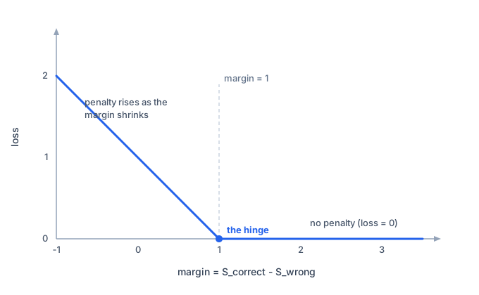
That corner at margin = 1 is where the loss switches from “penalty” to “no penalty.” It’s also why the earlier examples behave the way they do: everything to the right of the corner pays nothing, and everything to the left pays more the further left it goes.

Softmax Loss

Another approach, called softmax loss (or cross-entropy loss), comes from probability theory.

Instead of just comparing two scores, it asks: “If I treat the scores as probabilities, how likely is the correct label?”

First, convert scores to probabilities using the softmax function (this is a standard trick in statistics):

# exp(x) = e (about 2.718) raised to the power x.
# It turns any score, positive or negative, into a positive number.
#   exp(0) = 1
#   exp(1) = 2.718
#   exp(2) = 7.389
#   exp(-5) = 0.0067

probability_cat = exp(score_cat) / (exp(score_cat) + exp(score_dog) + exp(score_bird))

This converts any scores into numbers between 0 and 1 that sum to 1 (like probabilities).

Then the loss is:

# log(x) is the reverse of exp: it undoes it, so log(exp(x)) = x.
# The minus sign makes a low probability cost a lot and a high one cost little.
#   -log(1)   = 0      (perfectly confident and correct: no loss)
#   -log(0.9) = 0.1    (small loss, good)
#   -log(0.1) = 2.3    (large loss, bad)

# cat is the correct label in this example, so the loss uses probability_cat
loss = -log(probability_cat)

So the logarithm penalizes low-probability predictions harshly and rewards high-probability predictions gently.

Now run the same three scenarios through it.

Scenario B (confident): cat = 100, dog = 1, bird = 0.5. exp(100) is astronomically larger than the other two, so nearly all the probability lands on cat:

P(cat) ≈ 1.00
loss = -log(1.00) ≈ 0

Scenario A (close): cat = 10, dog = 9.5, bird = 8.

exp(10) = 22026,  exp(9.5) = 13360,  exp(8) = 2981   (sum = 38367)

P(cat) = 22026 / 38367 = 0.57
loss = -log(0.57) = 0.56

Cat wins, but because dog is close, cat gets only 57% of the probability, so there’s a real penalty.

Scenario C (wrong): cat = 3, dog = 10, bird = 1.

exp(3) = 20,  exp(10) = 22026,  exp(1) = 2.7   (sum = 22049)

P(cat) = 20 / 22049 = 0.0009
loss = -log(0.0009) = 7.0

Cat gets almost none of the probability, so the loss is large.

The numbers differ from hinge loss, but the ranking is the same: the confident call pays about nothing, the close call pays a little, the mistake pays a lot.

Which Loss Function Is Right?

Hinge loss (SVM) and softmax loss are different, and they lead to slightly different learned weightsthe numbers inside the model that it adjusts as it learns.. There’s no universal “right” answer; it depends on your problem and your preference.

Softmax has become more popular in deep learning for a couple of reasons.

First, it outputs a full set of probabilities (one per label, all adding up to 1), which is often useful on its own. A probability is a confidence figure on a fixed 0-to-1 scale, so you can act on it:

• Send anything below, say, 0.9 to a human to double-check.
• Weigh a costly mistake against a cheap one: flag a possible tumor even at 30% likelihood.
• Present a ranked list like “70% cat, 25% dog, 5% bird.”

Raw scores can’t support any of that, because their size carries no consistent meaning.

Second, softmax keeps giving a gentle learning signal even when a prediction is already correct, nudging the scores a little further apart, while hinge loss stops entirely once the correct label wins by the margin (that’s the flat part of the graph above). A loss that keeps offering feedback is a little easier to train with.

Hinge loss is still interpretable and useful in some contexts, such as traditional SVM classifiers.

The main point isn’t which one you choose; it’s that you need a loss function to:

1. Measure wrongness as a continuous number (not just right/wrong)
2. Give you a signal to optimize: “Make this number smaller”
3. Reward confident correct predictions and penalize confident wrong ones

The Whole Process

Here are all the steps together:

1. Compute scores (Part 5)
2. Measure loss (this post)
3. Adjust weights to reduce loss (next post: gradient descent)
4. Repeat

Gradient descent, in the next post, reads that loss to work out which direction to adjust each weight, and by how much.

Where These Formulas Come From

For where the above formulas actually come from (why the max, why the +1, why raise e to a power instead of just taking an absolute value), I wrote a separate side note that works through each piece: Why Do Hinge Loss and Softmax Look the Way They Do?

What’s Next

We have scores. We have a measure of wrongness. Now we need the algorithm that adjusts the weights to make that wrongness smaller. That’s gradient descent, a central optimization method used throughout machine learning.