Paper #1, Part 2: The Problem of Classification
Given a grid of numbers, name what the picture shows. It sounds simple. Seven specific things make it one of the hardest problems computers ever faced.
Where we are: Part 1 showed that an image is just a grid of numbers to a computer. Now we ask the actual task: given those numbers, how do we label the picture?
In the last post, we established the one idea this whole series stands on: to a computer, a picture is a grid of numbers. That post opened the file and showed them.
Now comes the task CS231n spends a semester on: image classification. The goal is simple to state:
Given an image (a grid of numbers), assign it a label from a fixed list of choices.
For example:
- Is this a picture of a cat or a dog?
- Is this a photograph of a car, a bike, or a truck?
- Does this X-ray show a broken bone: yes or no?
A human brain does this instantly and without effort. For a computer it is hard, hard enough that the seven challenges below are the reason simply comparing grids of numbers fails on real-world photos.
The Seven Things That Make It Hard
CS231n, formally titled “Convolutional Neural Networks for Visual Recognition,” is Stanford’s course on deep learning for computer vision. It opens with a list of challenges. Each one is a way that two pictures of the same subject end up with wildly different numbers.
Viewpoint variation. A dog viewed from the front looks different from a dog viewed from the side. A dog lying down looks different from a dog standing. The dog is still a dog, but the grid of numbers changes completely depending on where the camera is. Concretely: rotate the camera 90 degrees around the dog, and nearly every value in the grid changes, even though it’s the same animal.
Scale variation. A dog in the foreground of a photo takes up most of the image. A dog in the distance is tiny. Same dog, vastly different numbers.
Deformation. Dogs move. They stretch, crouch, and tilt their heads. The shape changes, so the numbers change.
Occlusion. Part of the dog might be hidden behind a tree or a person. Think of a dog photographed behind a picket fence, with only slivers of fur and one eye visible. The computer sees an incomplete picture but still has to produce the correct label, relying on whatever visible patterns it has learned to associate with “dog.”
Illumination conditions. A dog in bright sunlight produces completely different numbers than the same dog in shadow or under indoor lighting. The dog’s fur reflects light the same way it always did; what the camera records is the combination of that fur and the light hitting it.
Background clutter. If the dog is sitting in a park, the background is a mess of trees and grass. The computer has to separate the numbers that belong to “dog” from the numbers that belong to everything else. That’s surprisingly hard.
Intra-class variation. A Chihuahua and a Great Dane are both dogs, but they look almost nothing alike. Think of a Poodle, a Bulldog, and a Dalmatian: three dogs that share almost no obvious visual features, yet all belong to the same class. The computer needs to find the common thread underneath huge visual variation.
Why This Matters
Many image-classification methods are designed specifically to handle these seven kinds of variation.
A naive approach, comparing the number grids directly, fails in general for exactly the seven reasons above, though it can still work in narrow, controlled cases like matching a fixed logo photographed under identical lighting and angle every time. If you have a reference picture of a dog and you go looking for other pictures with identical numbers, you’ll fail constantly: viewpoint, lighting, occlusion, and a hundred other things will have changed the grid.
We need methods whose predicted label stays correct even when the picture changes. Methods that say “yes, this is a dog” even when the dog is rotated, occluded, far away, or in shadow.
This is what CS231n teaches us to build, one idea per post: first nearest neighbor (guess by finding the most similar stored example), then linear classifiers (score each possible label with a simple weighted recipe), then the convolutional networks built to handle these challenges.
The Same Dog, Different Numbers
The last post introduced this 64 × 64 cartoon dog and its file of numbers:

Here is the same dog, just moved down and to the right, and the same dog behind a fence:
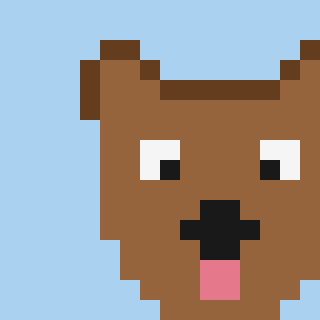
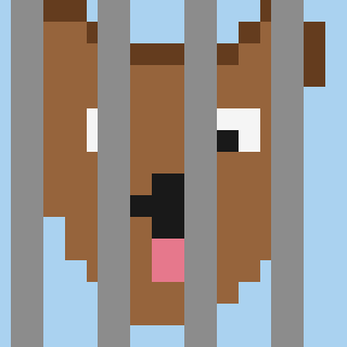
Here are their number files, to compare side by side with the original:
- dog-moved.ppm.txt: the dog only shifted position, yet more than half the numbers in the file changed. Every pixel the dog moved onto, and every pixel it moved off of, has new values.
- dog-fence.ppm.txt: the fence shows up as stripes of
140 140 140. Those gray columns replaced whole stretches of dog numbers.
To a person, all three pictures show the same dog. To a program comparing numbers, they barely agree. A classifier has to answer “dog” for all three anyway. Each of the seven challenges is one more way the numbers can change while the dog stays the same.
What’s Next
In the next post, we’ll try the simplest possible approach to classification anyway: find the stored image whose numbers are closest, and copy its label. It won’t work well. But it fails in a way that teaches us exactly what better methods need to do.
New terms from this series are collected in the glossary.