Paper #3: The Evidence (18 Layers vs. 34)
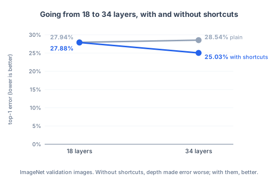
The same two networks from the first post, rebuilt with shortcuts. Without them, going from 18 to 34 layers made error worse. With them, it made error better by about three points.
Where we are: in a residual block, the layers learn only a change to their input, and a shortcut adds the input back. This post checks whether that fixed the problem from the first post.
The comparison
The authors ran a controlled test. They took their 18-layer and 34-layer plain networks, the pair where depth made things worse, and added a shortcut around every pair of layers. Nothing else changed: same layers, same training setup, and, because the shortcuts have no weights, the same number of weights. The paper calls the shortcut versions ResNet-18 and ResNet-34.
Here is top-1 error on the ImageNet validation images, the share of images where the network’s single best guess was wrong:
Reading across:
- Without shortcuts, adding 16 layers raised error from 27.94% to 28.54%.
- With shortcuts, adding the same 16 layers lowered error from 27.88% to 25.03%, a drop of about 2.8 points.
- At 34 layers, the version with shortcuts beat the plain one by about 3.5 points.
At 34 layers, the same comparison in top-5 error went from 10.02% without shortcuts to 7.76% with them.
With shortcuts, the deeper network did what depth was supposed to do. The training data agreed: the authors report that the 34-layer residual network “exhibits considerably lower training error” than the 18-layer one, the reverse of what happened with the plain networks. In the paper’s training curves (plots of error over the course of training), the 34-layer plain network’s error sits above the 18-layer one for the entire run; with shortcuts, the 34-layer curve ends up below.
At 18 layers, the two versions were nearly tied (plain 27.94%, with shortcuts 27.88%). The authors note that the residual version still helped there in a different way: it “converges faster,” reaching its final accuracy sooner. Their reading is that at 18 layers, ordinary training could still find a good solution for the plain network; the shortcuts mattered most once the network got deeper.
The same pattern on CIFAR-10
The authors repeated the test on the small CIFAR-10 dataset, where training is cheap enough to try many depths. Plain networks got worse as they got deeper; a 110-layer plain network had more than 60% error, enough that the paper leaves it off its chart. Residual networks kept improving with depth: 8.75% error at 20 layers, 7.51% at 32, 7.17% at 44, 6.97% at 56, and 6.43% at 110.
Did the layers learn small changes?
The hypothesis from the last post was that residual layers would only need to make small adjustments to what came in. The authors checked this on CIFAR-10 by measuring how strongly each layer responded, the standard deviation of its outputs, in plain and residual networks.
In a residual block, that output is the change the layers add to x before the shortcut adds x back, so a weak response means a small change. The residual layers responded more weakly than the plain ones. And the deeper the residual network, the smaller each layer’s response: in the paper’s words, “an individual layer of ResNets tends to modify the signal less.”
That is what the hypothesis predicts. In terms of the artists from the last post: each artist drew lightly on top of the drawing they received, and the longer the line, the lighter each artist’s marks. This supports the explanation without proving it, and the paper words it that way: the measurements “support our basic motivation.”
Same cost, better result
The comparison held one more thing equal. Adding x back costs one addition per number, which is negligible next to the multiplications inside the layers. The residual networks used the same number of weights and almost the same amount of computation as the plain ones. The improvement came from how the layers were connected, not from more resources.
What’s next
Thirty-four layers was a test. The next post is about how the authors went to 152 layers while keeping the computation manageable, using a cheaper kind of block called a bottleneck block.