Paper #3: Going to 152 Layers (The Bottleneck Block)

Where we are: shortcuts let a 34-layer network beat an 18-layer one. The authors then went much deeper, to 50, 101, and 152 layers. Doing that with the blocks from the earlier posts would have been expensive, so they designed a different block.

The cost of a convolution

A convolutional layer runs many filters across a stack of feature maps, and each filter spans the full depth of that stack. So a layer’s cost grows with how many maps go in and how many come out. A 3×3 layer that takes 256 maps and produces 256 has 3 × 3 × 256 × 256 = 589,824 weights, and it applies all of them at every position in the image.

Later in the network, closer to the answer, the stacks are wide: 256 maps or more. That comes from the rule in the first post, where each halving of the maps’ width and height doubles the number of filters. Stacking many layers that wide gets expensive fast.

The 1×1 convolution

The tool for cutting that cost is a filter only one position wide. A familiar example is turning a color photo into grayscale. A color image has 3 maps: red, green, and blue. At each pixel, grayscale takes the 3 values and combines them into 1, for example 0.30 × red + 0.59 × green + 0.11 × blue. Doing that at every pixel turns 3 maps into 1. That is a 1×1 convolution with 3 weights.

Inside a network it works the same way, on feature maps instead of colors, with weights the network learns. One 1×1 filter takes the 256 values at a position, one from each map, multiplies each by its own weight, and adds them up into 1 new value. Doing that at every position makes 1 new map.

Each filter makes one new map, so the number of filters sets how many maps come out. Grayscale is 1 filter, so 3 maps in gives 1 map out. A 2nd filter with different weights, say red minus green, would fill in a 2nd map, so 2 filters give 2 maps. In the same way, 64 filters reading 256 maps produce 64 maps. A separate set of 256 filters, with their own weights, then turns those 64 into 256 new maps.

Note that these 256 new filters don’t recover the original 256 maps; that information is already gone, just as a grayscale photo can’t give back the colors. They only produce the right number of maps for the shortcut to add the original input back.

Because it never looks at neighboring positions, a 1×1 filter can’t find patterns across space, like an edge. All it does is mix the maps at each position and change how many there are.

The bottleneck block

The new block, called the bottleneck block, has three layers instead of two, and two of them are the 1×1 layers introduced above:

1. a 1×1 layer that shrinks 256 maps down to 64,
2. a 3×3 layer that does the pattern-finding on just those 64,
3. a 1×1 layer that expands the 64 back to 256.

The shortcut still carries the original input around all three layers and adds it back (except at blocks where the number of maps changes, covered below). The block is called a bottleneck because its middle is narrow, the way a bottle narrows at the neck. The narrowing is what saves computation: the expensive 3×3 layer runs on 64 maps instead of 256.

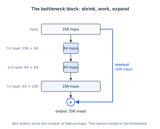
The savings are large. This three-layer block has 69,632 weights (16,384 + 36,864 + 16,384). The two-layer block from the earlier posts, used on just 64 maps (the comparison the paper makes), has 73,728. So the bottleneck handles four times as many maps at about the same cost. The authors describe the choice as “mainly due to practical considerations”: an engineering choice that makes more depth affordable.

152 layers, cheaper than 19

Using only bottleneck blocks in place of ResNet-34’s two-layer blocks, the authors built ResNet-50, ResNet-101, and ResNet-152. Each bottleneck block is 3 layers, so ResNet-50, for example, is 16 blocks (48 layers) plus the first and last layers. The 152-layer network needs 11.3 billion operations (multiply-adds) to process one image. VGG-16 needs 15.3 billion and VGG-19 needs 19.6 billion. So ResNet-152 is eight times as deep as VGG-19 and needs about 58% of the computation.

Error kept dropping as they went deeper. Measured the same way as the 18- and 34-layer results, by averaging the predictions over ten crops of each test image as AlexNet did, top-1 error was 22.85% for ResNet-50, 21.75% for ResNet-101, and 21.43% for ResNet-152, down from 24.52% for the 34-layer network, which used the same kind of shortcut but the original two-layer blocks.

When the shortcut needs help

In the example from the post on residual blocks, 5.0 came in, the layers produced 0.2, and the shortcut added the two: 5.2. In a real network, x isn’t a single number. It’s a stack of feature maps, each one a grid of numbers. The shortcut adds the two stacks number by number: the 1st map of x to the 1st map of the layers’ output, position by position, then the 2nd map to the 2nd, and so on. With 2 maps of 2 positions each:

x:              map 1 = [5.0,  3.0]   map 2 = [1.0, 4.0]
layers' output: map 1 = [0.2, −0.1]   map 2 = [0.0, 0.3]
sum:            map 1 = [5.2,  2.9]   map 2 = [1.0, 4.3]

That pairing only works when both stacks have the same number of maps. At the first block of each new stage, they don’t. In ResNet-34, one such block takes in 64 maps and its layers put out 128, so maps 65 through 128 have nothing in x to be added to. (These blocks also halve the maps’ width and height; the shortcut handles that by keeping every other row and every other column.)

The paper tried three fixes on the 34-layer network:

• Pad with zeros: add 64 all-zero maps to the shortcut so it carries 128. No new weights, but maps 65 through 128 then get nothing added, so the paper notes they have “no residual learning.” 25.03% top-1 error.
• A 1×1 convolution where sizes change: a 1×1 layer with 128 filters, like the ones above, turns the shortcut’s 64 maps into 128. This adds weights only at the 3 blocks that change size. 24.52%.
• A 1×1 convolution on every shortcut, even where sizes already match, adding weights at 13 more blocks. 24.19%.

All three are within about 0.8 points of each other, and all three beat the plain 34-layer network’s 28.54% by 3.5 points or more. The authors conclude that the extra weights “are not essential for addressing the degradation problem.” The deeper networks use the middle option.

What’s next

The last post looks at what these networks won, where going deeper stopped helping, and how this paper leads into the next one on the list.