Paper #1, Part 16: Putting It Together (What CS231n Actually Teaches)

Where we are: over fifteen posts we have built every piece, from pixels to trained convolutional networks (Parts 1 to 15). This post puts them together into one complete image classifier.

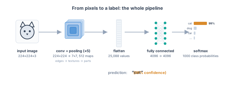
Let’s trace a complete example: classifying a cat image.

The Pipeline

Step 1: Input

Raw image: 224×224 pixels, each with 3 color channels (RGB), so the input is a 224×224×3 block of values, each from 0 to 255.

First thing: normalize. Divide by 255, or standardize using ImageNeta large public image dataset networks are commonly pre-trained on. statistics. Normalized image: same shape, values now on a sensible scale.

Step 2: Early Convolutions

First convolutional layer: 64 filtersa small grid of weights that detects one pattern (also called a kernel)., each detecting simple patterns (edges, corners, colors).

Each filter spans all three color channels: a 3×3 filter is really 3×3×3, covering a small patch across red, green, and blue at once. Slide it across the image, and at each position it multiplies those 27 values by its weightsthe numbers inside the model that it adjusts as it learns. and sums them into a single number. So one filter produces one 2D feature mapthe grid of responses a filter produces as it slides over the input., not three. (This is the same depth-spanning idea from Part 12, where a deeper filter spans all the feature maps beneath it; here the depthhow many layers are stacked in the network. is just the 3 color channels.)

Output: 64 feature maps, 224×224. (Padding the edges keeps the size the same; without paddinga border of zeros around the image so the output keeps its size. it would be 222×222.)

Apply ReLUan activation that keeps positive values and sets negatives to zero. activation: set negative values to zero, leave positives unchanged.

Pool with 2×2 max poolingkeep the largest value in each small region.: output becomes 112×112.

Result: 64 feature maps of edges and simple patterns.

Step 3: Intermediate Convolutions

Second convolutionslide a small filter across the image to find a pattern anywhere.: 128 filters, applied to the 64 input maps.

These filters detect combinations of edges: textures, blobs, more complex patterns.

Output: 128 feature maps, 112×112.

ReLU, then 2×2 poolingdownsample a region to one value, shrinking the feature maps.: 56×56.

Repeat: more convolutions, more pooling, increasing complexity and decreasing size.

By layer 5: perhaps 512 feature maps, 7×7.

Each map detects high-level concepts: object parts, shapes, semantic features.

Step 4: Classification

Flatten the 512×7×7 maps (unroll the whole 3D block into one long list) into a vector: 512 × 49 = 25,088 values.

Pass through fully-connected layersa layer where every input connects to every neuron.:

• Dense layer 1: 4096 neuronsone unit that weights its inputs, adds them up, and applies an activation., ReLU
• Dense layer 2: 4096 neurons, ReLU
• Output layer: 1000 neurons (one per ImageNet category)

During training, dropoutrandomly switch off neurons during training so none becomes essential. (randomly zeroing 50% of the neurons) is applied to these dense layers to prevent overfittingmemorizing the training data instead of learning general patterns..

Apply softmaxturns raw scores into probabilities that add up to 1., which turns the raw scores into probabilities that add up to 1. If the cat is clearly visible, the “cat” neuron fires strongest, and softmax returns ~0.99 for cat, ~0.01 split among others.

Step 5: Inference

The predicted class is whichever output neuron has the highest probability (its argmax), here “cat”.

Network predicts “cat” with 99% confidence.

Why This Works

Hierarchy: Early layers learned low-level features (edges). Middle layers combined them into medium-level features (textures). Late layers combined those into high-level features (objects).

By the final convolutional layers, each location in the feature maps encodes something high-level, like “there’s a cat face around here.” The fully-connected layers then weigh all of that together to make the call.

Robustness: Pooling and convolutions make the network robust to small shifts. A cat’s whiskers don’t have to be at pixel-perfect positions.

Generalization: Regularization (dropout, and weight decaya penalty on large weights (also called L2 regularization)., a penalty on large weights) prevents the network from memorizing specific training images. It learns generalizable patterns.

Transfer learning: If you’re fine-tuningkeep training the reused layers, gently, on your own data. a pre-trained network, the early layers already recognize edges and textures. You only need to train the late layers to recognize your specific categories.

Why CS231n Matters

CS231n teaches this entire pipeline from scratch. You don’t just use a library; you understand:

• Why architecture matters
• Why data preparation matters
• Why regularizationtechniques that hold a model back so it generalizes better. matters
• How backpropagationthe method that computes the gradient for every weight at once. trains weights
• What the network actually learns

This understanding transfers to other domains. Ideas move between fields: the transformer, the architecture behind modern language models like ChatGPT, was later adapted to images too. And principles like overfitting and regularization apply everywhere.

CS231n is foundational because it builds intuition. Once you understand how a CNN works, adapting it to new tasks or understanding new architectures is straightforward.

The Journey

Fifteen posts ago, image classificationsorting an input into one of a fixed list of labels. was a black box. Here’s the ground we’ve covered since:

• How computers represent images as numbers
• Why nearest neighborlabel a new image by copying its most similar training image. fails
• How linear classifiersscores an image with a weighted sum of its pixel values. score images
• How loss functionsthe rule that turns the guesses and answers into the loss number. measure wrongness
• How gradient descentrepeatedly nudge the weights downhill to shrink the loss. optimizes weights
• How backpropagation computes gradientsthe slope of the loss for each weight: which way, and how steeply. efficiently
• How neural networks with activation functionsa simple bend applied to a neuron's output, like ReLU. learn non-linear patterns
• How convolutions exploit locality
• How pooling builds hierarchies
• How regularization prevents overfitting
• How to visualize what networks learn
• How to reuse trained networks

This is deep learning. We’ve now followed the whole path, from representing an image as numbers to a working image classifier.

Going further means building something: take a pre-trained model off the shelf (a ResNet, which is a deep CNN, or a Vision Transformer, ViT), fine-tune it on new data, and deploy it. The ideas from this series carry over directly.