Paper #2: Fighting Overfitting at Scale
With sixty million weights and only a million images, AlexNet could have memorized its way to a useless answer. Two defenses stopped it: more data, made for free, and dropout.
Where we are: ReLU made training fast, and splitting across two GPUs made it fit in memory. This post is about the remaining problem: with 60 million weights, the network could simply memorize its training set instead of learning from it.
Paper #1 called this overfitting: a network with enough capacity learns the training images by heart, scores beautifully on them, and then fails on anything new. AlexNet had plenty of capacity and only 1.2 million images to feed it.
Why more weights make memorizing possible
Each weight, and each bias, is a knob that training turns. The number of knobs decides how many images a model can sort correctly no matter how they are labeled, and that is what makes memorizing possible. The simplest case, a straight boundary, shows how.
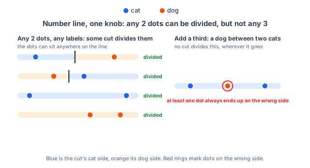
One axis, one knob. Put each image on a number line. The boundary is a single cut point, and its one knob slides the cut left or right. Either side can be the cat side. Any two images, wherever they fall and however they are labeled, can be divided by some cut. That’s not the case with three coin flips. Sooner or later they come up cat, dog, cat: a dog with a cat on each side. No cut divides that.
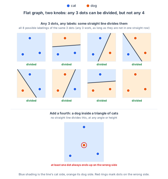
Two axes, two knobs. On a flat graph, like the one in Paper #1’s first post, the boundary is a straight line, with one knob to turn it and one to slide it. Any three images, as long as they do not sit in one straight row, can be divided however they are labeled. That’s not the case with four coin flips: sooner or later the labels come out in a way no straight line can divide, such as a dog inside a triangle of cats.
Three axes, three knobs. In a room, the boundary is a flat pane, with two knobs to tilt it and one to raise or lower it. Any four images, as long as they do not all lie on one flat sheet, can be divided. That’s not the case with five coin flips: sooner or later the labels come out in a way no pane can divide, such as a dog inside a pyramid of cats.
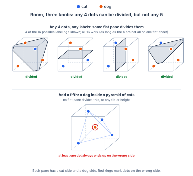
The pattern holds at every size: a boundary with N knobs can divide any N + 1 images, however they are labeled, but not every set of N + 2. So when there are relatively few images compared to the number of knobs, any labels fit, even coin flips, and a perfect score proves nothing. When images far outnumber the knobs, most labelings cannot be fit, so a boundary that does fit them has almost certainly found a real pattern.
An image has far more than three axes: one per pixel value, 3,072 for a tiny 32 × 32 color image, with a knob for each. A flat boundary with that many knobs can divide about 3,000 images any way at all. Give it 1,000 training images labeled by coin flip, pure noise, and it can still sort them perfectly. A model that can fit random labels is not finding patterns; it has enough freedom to fit anything. That is memorization.
There is a second way a model gets this kind of freedom. Activation functions, like the ReLU from two posts back, let the boundary bend, and more neurons mean more bends, enough for the boundary to wind around individual images. Everything above uses straight boundaries to keep the picture simple, so this post leaves bends aside.
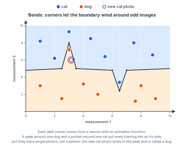
What matters is knobs compared to data. As we showed above, even the two-knob line can fit any labels on three dots. AlexNet had about 60 million weights for 1.2 million images, roughly 50 knobs per image: plenty of freedom to store details of individual images instead of patterns shared across them. Left alone, it would overfit badly. The authors leaned on two defenses.
Defense one: more data, made for free
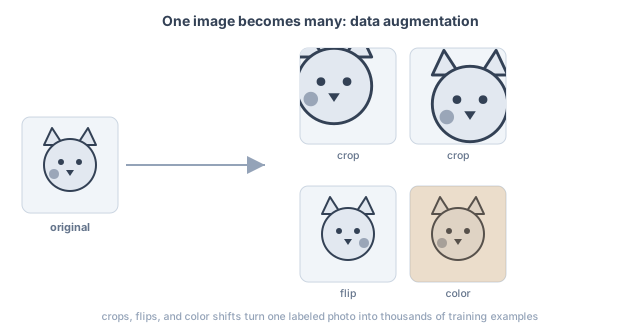
The most direct way to reduce overfitting is more training data, because quirks are harder to memorize across a larger, more varied set. You rarely have more data lying around, so AlexNet created more from the images it already had, a trick Paper #1 introduced as data augmentation. AlexNet used two kinds.
The first is familiar: take random smaller crops of each image, and flip some of them left-to-right. A dog is still a dog when it is shifted a little or mirrored, so each original photo can yield over two thousand slightly different training examples. They are close copies of each other, as the authors note, but each one shows the network a slightly different view, without taking any new photos. At test time the network steadies its answer by averaging its predictions over ten fixed crops of each image.
The second is newer and worth a closer look: color jitter. The authors nudged the overall color and brightness of each image at random, but not arbitrarily. They measured how colors naturally vary across the whole dataset and shifted along those same directions, so the changes looked like plausible lighting differences rather than random noise. This taught the network that a dog is a dog whether the photo is warm or cool, bright or dim. It cut the top-1 error (how often the single best guess is wrong) by more than one percentage point on its own. A single percent sounds small, but on a benchmark decided by a point or two, it was well worth a trick that costs almost nothing to apply.
Defense two: dropout
The second defense was dropout, which Paper #1 explains in detail: during training, randomly switch off half the neurons on each pass, so the network cannot lean on any single one and has to spread what it learns across many.
AlexNet’s specifics are worth noting. It used dropout at a rate of 50%, and only in the first two fully-connected layers, which is where most of those 60 million weights live and where overfitting had the most room to happen. At test time, dropout is switched off and the full network makes the prediction, with a small adjustment so the totals still line up (Paper #1 covers that bookkeeping). The cost during training is that dropout roughly doubles the number of passes needed to finish. The authors judged that a fair price: without dropout, they report, the network overfit substantially.
The payoff
Dropout was brand new in 2012, and AlexNet was among the first to put it to serious use; the color jitter was AlexNet’s own invention; only the crops and flips were an established idea. What AlexNet showed was that these defenses, used together at this scale, were enough. Paper #1 can teach them as fundamentals today partly because this paper showed they worked.
What’s next
The large pieces are now in place: a fast activation, a way to fit the model in memory, and a working defense against overfitting. The next post gathers up the smaller tricks the paper used, and the plain hard work of actually running the training.