Paper #6: How an RNN Remembers
An RNN's memory is a list of numbers. At each step it mixes that list with the new input to make an updated list, using the same weights every time. The network repeats this once for each character it reads.
Where we are: the last post introduced recurrent networks, which read a sequence one piece at a time. This post covers what their memory is and how it changes at each step.
The memory is a list of numbers
An RNN’s memory, called its hidden state, is a list of numbers. In Karpathy’s small teaching example, the list has 3 numbers. In the networks he trains on real text, it has 512 per layer.
Before the 1st step, every number in the list is 0. At each step, the network reads one new input, such as one character, and computes a new list from 2 things: the new input and the list it had before. The new list replaces the old one. Whatever the network needs to remember about the sequence so far has to be held in those numbers. The list has a fixed length, so a long sequence has to be squeezed into the same few hundred numbers, and some of it gets lost.
This post describes the plain RNN, the simplest version. Karpathy’s experiments use a more complex variant, the LSTM, covered at the end, but it has the same overall shape.
One step
Karpathy writes the step as a few lines of code. In words, the update is:
new memory = tanh( memory weights × previous memory + input weights × new input )
Taking the parts one at a time:
- memory weights × previous memory. Each new memory value starts as a weighted sum of all the previous memory values, the same kind of weighted sum a linear classifier uses. This is how the past carries forward.
- input weights × new input. A 2nd weighted sum, this time of the new input’s values, is added on. This is how the new character gets in.
- tanh. The total for each value is passed through tanh, an S-shaped curve that squeezes any number into the range −1 to 1. Without it, the values could keep growing as the step repeats. Paper #2 covered tanh as an activation function.
The output at each step comes from the new memory, through a 3rd set of weights:
output = output weights × new memory
When the network is predicting text, the output is one score for each possible next character. The next post covers how the scores become probabilities.
The same weights at every step
The network repeats this step once for each character it reads, passing the memory from each step to the next:
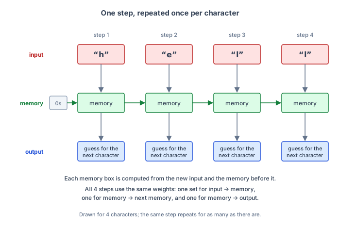
All the steps share the same 3 sets of weights: input to memory, memory to memory, and memory to output. A network trained on sentences of 50 characters can still run on a sentence of 500, because it never had a separate set of weights for each position.
Karpathy compares this to a computer program. A regular network works like a function: the same input always gives the same output, whatever it was given before. An RNN works more like a program that keeps variables as it runs. Its memory values change with each character it reads, so the same character can lead to a different output depending on what came before. The weights decide how that program behaves, and training adjusts them.
Training: unroll, then pass the blame back
The weights start as small random numbers. Training adjusts them the same way as in Paper #1: measure how wrong the outputs are with a loss, then use backpropagation to work out how to nudge every weight.
The difference is that the network has to be unrolled first, as in the figure. Once it’s drawn out step by step, it’s an ordinary network with many layers, one per step, that happen to share weights. Backpropagation runs back through the steps, from the last character to the 1st, collecting the error from every step’s prediction along the way. This is called backpropagation through time.
Long texts are cut into stretches for this. In Karpathy’s runs, the error is passed back through 100 characters at a time. The memory itself carries over from one stretch to the next; only the error stops at the 100-character boundary.
Stacking
RNNs can be stacked like the layers of any other network. In a 2-layer RNN, the 1st RNN reads the input characters, and the 2nd RNN reads the 1st one’s memory values as its inputs, one step at a time. Each has its own memory and its own weights. Only the top RNN’s output is turned into scores for the next character. Karpathy’s networks use 2 or 3 layers.
A note on LSTMs
Every experiment in Karpathy’s post uses an LSTM (long short-term memory), not the plain RNN above. An LSTM keeps the same outline: one step, repeated, passing its memory along, with the same weights each time. The differences are inside the step: the update is more complex, and the memory is 2 lists of numbers instead of 1, called the cell state and the hidden state. Karpathy says it “works slightly better in practice,” and doesn’t go into how.
The reason usually given is the problem from Paper #3, the vanishing gradient: passed back through many steps, the training signal can shrink until the early steps barely learn. The LSTM’s update is designed so that information, and the training signal, can pass through many steps with less loss than in a plain RNN. Paper #7, Christopher Olah’s “Understanding LSTM Networks,” covers how.
What’s next
The next post uses Karpathy’s 4-letter example to show how an RNN is trained to predict the next character, and how it then writes new text.