Paper #2: The Architecture (Everything from Paper #1, Scaled Up)

Where we are: last time we saw the contest AlexNet won and by how much. Now we look inside the network itself, which turns out to be familiar ground.

After Paper #1, AlexNet’s shape is already familiar. The main idea of this post: the architecture is not where the surprise is. It is the ordinary convolutional network from that series, built bigger than anyone had trained before.

Eight layers that learn

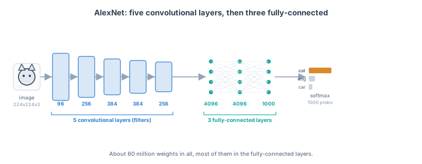
AlexNet has eight layers with weights: five convolutional layers followed by three fully-connected ones. An image goes in the front; a softmax at the end turns the final scores into probabilities across the 1,000 categories.

The input is a 224×224 color image, which is 224×224×3 numbers (one per color channel). (A small aside: the paper says 224×224, but the layer sizes only work out if the input is actually 227×227. It is a slip in the original that has puzzled readers ever since; 224 is the number the paper prints, so it is the one we will use.) From there:

• The five convolutional layers do the pattern-finding, exactly as in Paper #1. Early layers catch edges, later ones catch textures and object parts, the hierarchy we built up before. The first layer alone sweeps 96 different 11×11 filters across the image; deeper layers use smaller 3×3 and 5×5 ones. The filter count rises and then levels off: 96, then 256, then 384, 384, and 256. Pooling layers in between shrink the maps, so the picture gets smaller while the stack of feature maps gets deeper as you go.
• The three fully-connected layers at the end weigh all the evidence together to make the call. The first two have 4,096 neurons each; the last has 1,000, one per category.

The fully-connected layers hold most of the network’s weights. Wiring a few thousand inputs to 4,096 neurons takes tens of millions of weights in a single fully-connected layer, far more than the five convolutional layers put together (which hold only a couple of million between them). A convolution is frugal because it reuses one small filter everywhere; a fully-connected layer gives every connection its own weight.

The original AlexNet diagram in the paper appears split into two parallel halves. That split is not part of the core design. It is mostly a hardware workaround for the GPUs of 2012, which a later post covers in full.

Big for its time

Those layers add up to about 60 million weights and 650,000 neurons. In 2012 that was enormous: earlier networks trained on real images had at most a few million weights, and AlexNet had sixty million. Fitting and training that many, on 1.2 million images, is exactly why so much of the rest of the paper is about making training work at all.

Capacity like that is a double-edged thing, as Paper #1 warned: a network with 60 million knobs can memorize instead of learn. Holding that off is a theme of the posts to come.

Depth is not decoration

One finding is worth pulling out. The authors tried removing a single one of the middle convolutional layers, each of which holds less than 1% of the total weights. Accuracy dropped by about two percentage points each time.

So the depth matters. Two percentage points may not sound like much, but at this level it is a serious amount; at the time, teams were competing over fractions of a point. It is not that the network is big for the sake of being big; each layer builds on the patterns found by the one before it, and removing one weakens everything above it.

A fair question follows: if removing a layer hurts, why not add more? The authors were direct about the limit. The network’s size, they wrote, was capped by the memory on 2012’s GPUs and the training time they could tolerate; they expected their results to keep improving on their own as faster GPUs and bigger datasets arrived. They wanted bigger and could not get there yet.

The exact recipe, five convolutional layers and three fully-connected with those filter counts, was tuned by experiment, not derived from theory; the only structural claim the paper backs with evidence is the layer-removal test above. Going much deeper would have hit a different wall. Training works by passing a “how wrong you were” signal backward from the end of the network to the front, the process called backpropagation in Paper #1. Across dozens of layers that signal fades, like a photocopy of a photocopy, each copy a little fainter than the last, until the earliest layers barely change and stop improving. Fixes for that fading signal arrived over the next few years, and the next paper, ResNet, takes on the problem that remained after them.

What’s next

The shape, then, is the one from Paper #1. The challenge was training something this large without the training stalling or the network just memorizing its examples. The next post starts with the change that made the training fast enough to be possible at all.